SHAP summary (beeswarm)
Every school district's SHAP value for every characteristic, coloured by the characteristic's value, with mean |SHAP| importance.
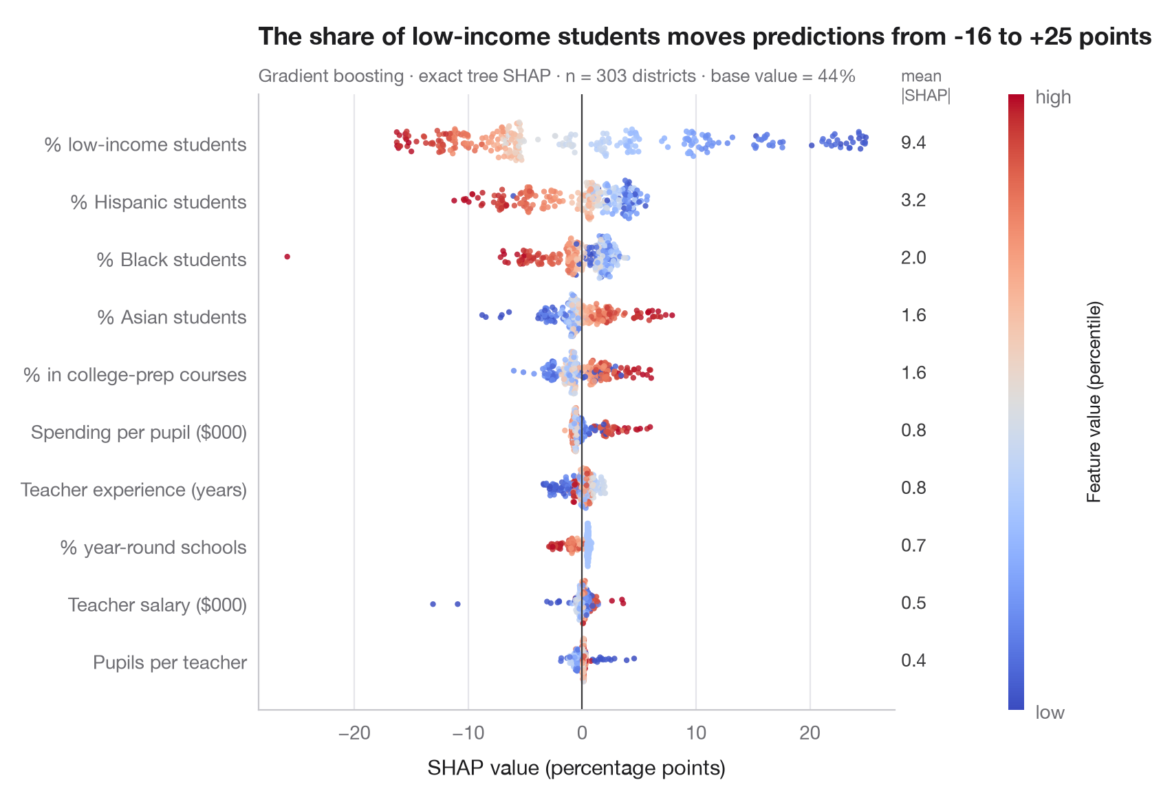
SHAP (SHapley Additive exPlanations; Lundberg and Lee, 2017) splits each prediction into additive contributions, one per feature, so that base value + sum of contributions = prediction. The contributions are Shapley values from cooperative game theory: each feature's average marginal effect over all orders in which features could be added.
The beeswarm shows one dot per school district and feature. Position is the SHAP value — how far that feature pushed this district's prediction up or down — and colour is the feature's own value, from low (blue) to high (red). Features are sorted by mean |SHAP|, printed on the right as a global importance. A clean red-right / blue-left split means a monotone effect; mixed colours signal non-linearity or interactions.
Data are the 303 California school districts of the 1998 STAR test bundled
with statsmodels (sm.datasets.star98); the outcome is the share of
students scoring above the national median in maths, in percentage points,
predicted from ten district characteristics. The model is a gradient-boosting
regressor and the exact tree SHAP values come from
shap.TreeExplainer. The figure is drawn with Matplotlib so it matches the
gallery style; shap.plots.beeswarm gives a similar view in one line.
import matplotlib.pyplot as plt
import numpy as np
import shap
import statsmodels.api as sm
from sklearn.ensemble import GradientBoostingRegressor

# Data: 303 California school districts; outcome = % of students above the national median in maths
d = sm.datasets.star98.load_pandas().data
y = 100 * d["NABOVE"] / (d["NABOVE"] + d["NBELOW"])
names = {"LOWINC": "% low-income students", "PERASIAN": "% Asian students", "PERBLACK": "% Black students",
         "PERHISP": "% Hispanic students", "AVYRSEXP": "Teacher experience (years)",
         "AVSALK": "Teacher salary ($000)", "PERSPENK": "Spending per pupil ($000)",
         "PTRATIO": "Pupils per teacher", "PCTAF": "% in college-prep courses",
         "PCTYRRND": "% year-round schools"}
X = d[list(names)]
model = GradientBoostingRegressor(learning_rate=0.05, n_estimators=300, max_depth=2,
                                  subsample=0.8, random_state=0).fit(X, y)

# Exact SHAP values for tree ensembles
sv = shap.TreeExplainer(model).shap_values(X)          # shape: (districts, features)
importance = np.abs(sv).mean(axis=0)
order = np.argsort(importance)                          # least important at the bottom

fig, ax = plt.subplots(figsize=(8, 5.6))
rng = np.random.default_rng(0)
cmap = plt.get_cmap("coolwarm")
for i, j in enumerate(order):
    v = sv[:, j]
    xv = X.iloc[:, j].rank(pct=True).to_numpy()         # colour = percentile of the feature value
    # Beeswarm-style vertical jitter: wider where the points are denser
    hist, edges = np.histogram(v, bins=60)
    dens = hist[np.clip(np.digitize(v, edges) - 1, 0, len(hist) - 1)] / hist.max()
    jitter = rng.uniform(-1, 1, len(v)) * 0.38 * np.sqrt(dens)
    ax.scatter(v, i + jitter, c=xv, cmap=cmap, s=9, alpha=0.85, lw=0, vmin=0, vmax=1)
    ax.text(1.01, i, f"{importance[j]:.1f}", transform=ax.get_yaxis_transform(), va="center",
            fontsize=9.5, color="#3A3A3C")
ax.axvline(0, color="#3A3A3C", lw=0.8)
ax.set_yticks(range(len(order)), [names[X.columns[j]] for j in order])
ax.set_xlabel("SHAP value (percentage points)")
ax.grid(axis="x"); ax.grid(axis="y", visible=False)
ax.text(1.01, len(order) - 0.35, "mean\n|SHAP|", transform=ax.get_yaxis_transform(),
        fontsize=8.5, color="#6E6E73", va="bottom")

cb = fig.colorbar(plt.cm.ScalarMappable(cmap=cmap), ax=ax, pad=0.09, aspect=40, ticks=[0, 1])
cb.ax.set_yticklabels(["low", "high"])
cb.set_label("Feature value (percentile)", fontsize=9.5)
cb.outline.set_visible(False)

low = sv[:, list(X.columns).index("LOWINC")]
ax.set_title(f"The share of low-income students moves predictions from {low.min():+.0f} to {low.max():+.0f} points", pad=26)
ax.text(0, 1.02, f"Gradient boosting · exact tree SHAP · n = {len(X)} districts · "
        f"base value = {model.predict(X).mean():.0f}%", transform=ax.transAxes, fontsize=9.5,
        color="#6E6E73")
plt.show()
Figures use the optional PyStatlas style: add plt.style.use("pystatlas.mplstyle") to match the look exactly.
Data source
- California STAR test results, 1998 (303 school districts). Gill, J. (2001). Generalized Linear Models: A Unified Approach (Quantitative Applications in the Social Sciences, No. 134). Sage. https://www.statsmodels.org/stable/datasets/generated/star98.html
Original data from the California Department of Education's Standardized Testing and Reporting (STAR) program, 1998. Subset distributed with statsmodels (sm.datasets.star98) with the author's permission.
The examples illustrate statistical methods. Their titles describe what each figure shows in these particular data — often a small, dated or partial sample — not the author's position on the substantive question. For interpretation, context and data quality, rely on the original sources cited here.
How to cite
PyStatlas is created and maintained by Thierry Warin. If it helped your work, please cite it.
Warin, T. (2026). SHAP summary (beeswarm). In PyStatlas: A Python Gallery of Statistical Graphics for the Social Sciences. https://warint.github.io/pystatlas/machine-learning/shap-beeswarm/
@misc{warin2026statlas,
  author       = {Warin, Thierry},
  title        = {PyStatlas: A Python Gallery of Statistical Graphics for the Social Sciences},
  year         = {2026},
  howpublished = {\url{https://warint.github.io/pystatlas/}},
  note         = {Source code: https://github.com/warint/pystatlas}
}More in Machine learning
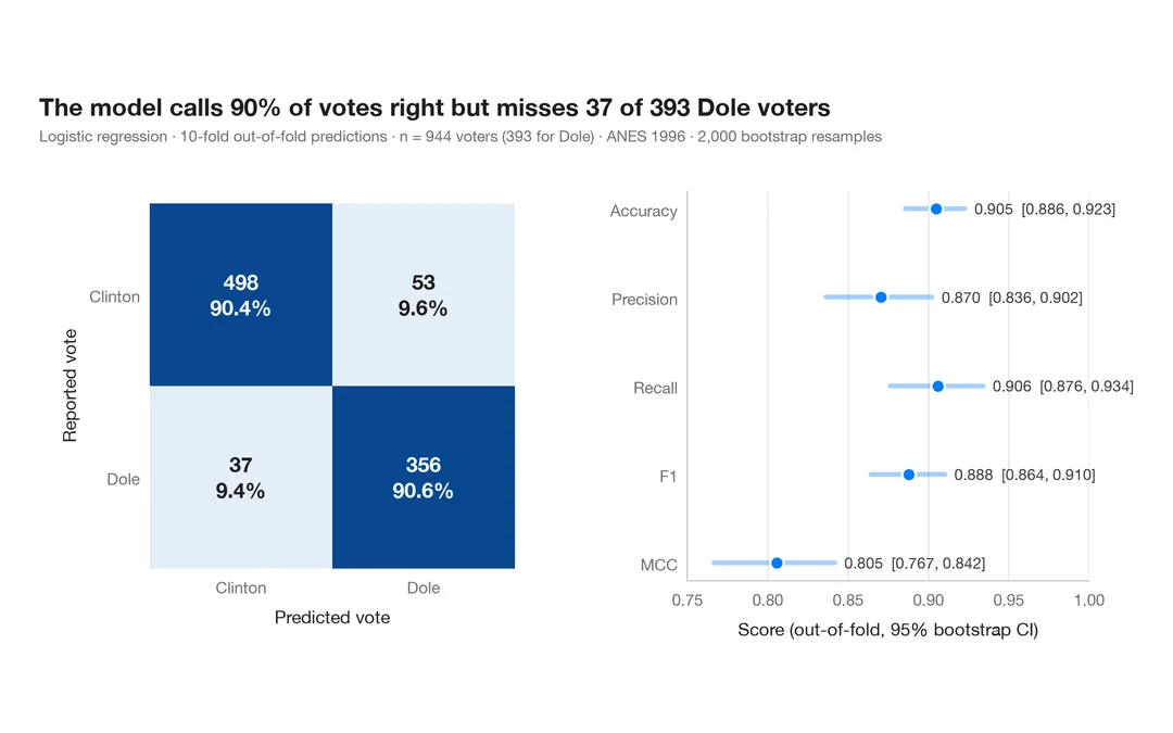
Confusion matrix with metrics
How well a logistic regression predicts who voted Dole in 1996 — out-of-fold confusion matrix with counts and row shares, and bootstrap intervals for the headline metrics.
yardstick::conf_mat() + autoplot()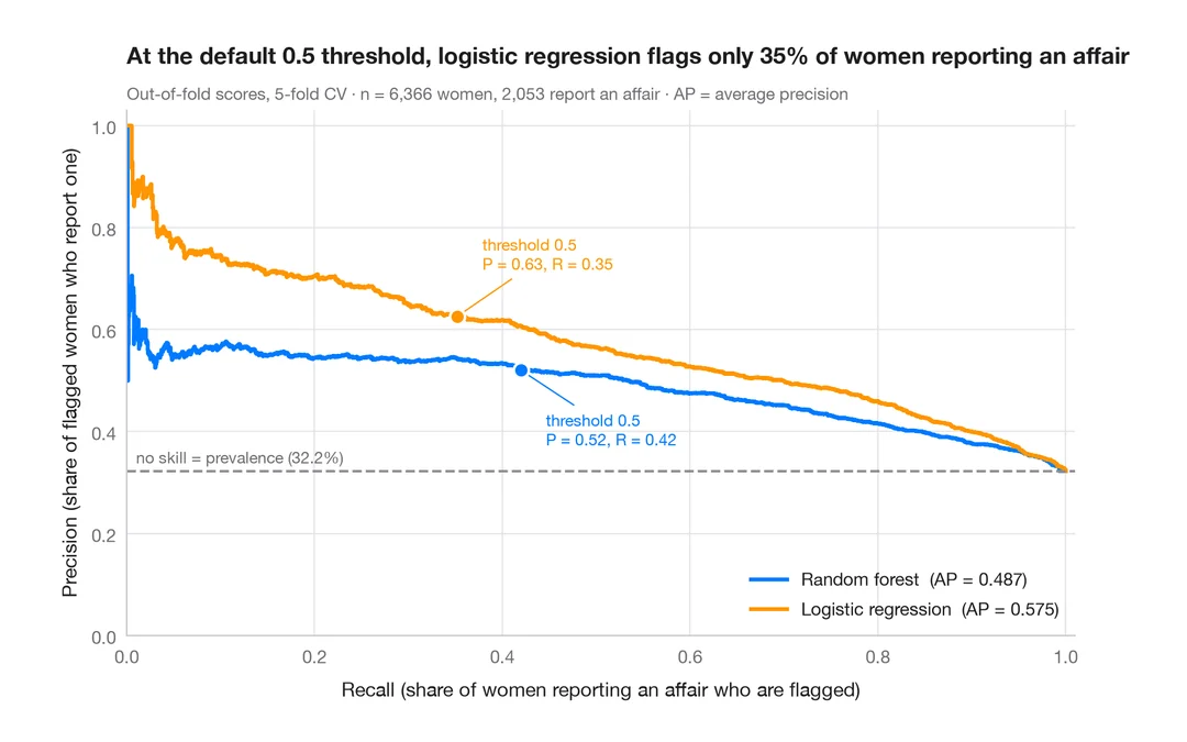
Precision–recall curves
Out-of-fold precision–recall curves for two classifiers predicting which married women report an affair, with average precision and the no-skill baseline.
yardstick::pr_curve() + autoplot()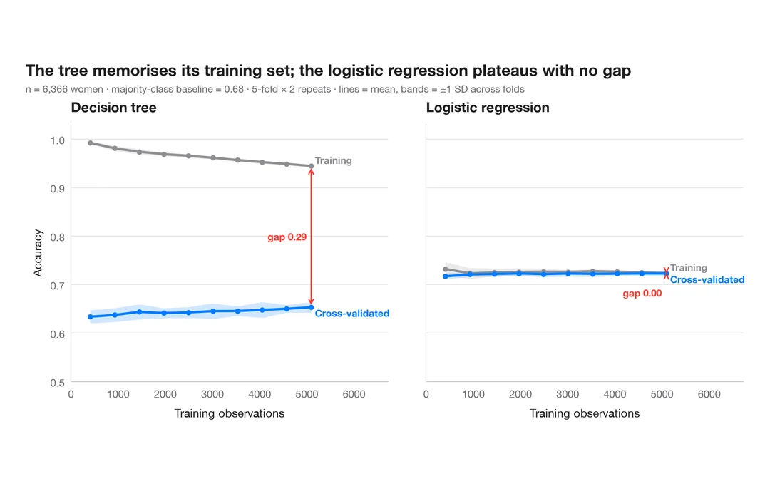
Learning curve
Training and cross-validated accuracy as the training set grows, for two models predicting which married women report an affair.
caret::learning_curve_dat() + ggplot()