Moran scatterplot (global autocorrelation)
Each area against the average of its neighbours, with Moran's I, its permutation test and the reference distribution.
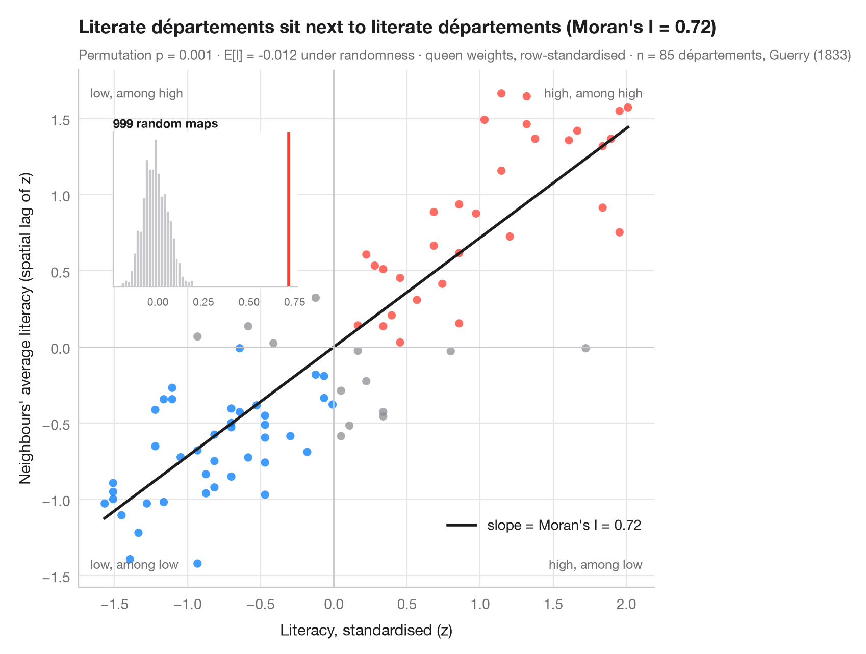
Global spatial autocorrelation asks one question for the whole map: do similar values sit next to each other more than chance would allow? The Moran scatterplot answers it visually. Each point is an area: on the horizontal axis its own (standardised) value, on the vertical axis the average of its neighbours — the spatial lag. With row-standardised weights, the slope of the fitted line is exactly Moran's I (Moran, 1950). Points in the upper-right and lower-left quadrants are areas that resemble their neighbours; the other two quadrants hold spatial outliers.
Inference is by permutation: the values are shuffled across the map 999
times and I is recomputed each time. The inset shows that reference
distribution under spatial randomness; the pseudo p-value is the share of
shuffles at least as extreme as the observed I. Data are Guerry's (1833)
literacy rates for 85 French départements, loaded with libpysal;
weights are queen contiguity and the statistic comes from esda.Moran.
import geopandas as gpd
import matplotlib.pyplot as plt
import numpy as np
from esda.moran import Moran
from libpysal import examples, weights

# Data: literacy of military conscripts in 85 départements, c. 1830 (Guerry, 1833)
g = gpd.read_file(examples.load_example("Guerry").get_path("guerry.shp"))
y = g["Litercy"].to_numpy(dtype=float)

# Row-standardised queen weights, Moran's I with 999 permutations
w = weights.Queen.from_dataframe(g, use_index=False)
w.transform = "r"
mi = Moran(y, w, permutations=999)
z = (y - y.mean()) / y.std()
lag = weights.lag_spatial(w, z)              # average of the neighbours' z-scores

fig, ax = plt.subplots(figsize=(8, 6.2))
quad = np.select([(z > 0) & (lag > 0), (z < 0) & (lag < 0)], ["#FF3B30", "#007AFF"], "#8E8E93")
ax.scatter(z, lag, s=34, c=quad, alpha=0.75, lw=0)
xs = np.array([z.min(), z.max()])
ax.plot(xs, mi.I * xs, color="#1D1D1F", lw=2, label=f"slope = Moran's I = {mi.I:.2f}")
ax.axhline(0, color="#C7C7CC", lw=1); ax.axvline(0, color="#C7C7CC", lw=1)
for (tx, ty, txt) in [(0.98, 0.97, "high, among high"), (0.02, 0.03, "low, among low"),
                      (0.02, 0.97, "low, among high"), (0.98, 0.03, "high, among low")]:
    ax.text(tx, ty, txt, transform=ax.transAxes, ha="right" if tx > 0.5 else "left",
            va="top" if ty > 0.5 else "bottom", fontsize=9, color="#6E6E73")
ax.set_xlabel("Literacy, standardised (z)")
ax.set_ylabel("Neighbours' average literacy (spatial lag of z)")
ax.grid(axis="x")
ax.legend(loc="lower right", bbox_to_anchor=(1, 0.08))

# Inset: reference distribution of I under spatial randomness
ins = ax.inset_axes([0.06, 0.58, 0.32, 0.3])
ins.hist(mi.sim, bins=30, color="#C7C7CC", edgecolor="white")
ins.axvline(mi.I, color="#FF3B30", lw=2)
ins.set_title("999 random maps", fontsize=8.5, loc="left", pad=3)
ins.tick_params(labelsize=7.5); ins.set_yticks([]); ins.grid(False)

ax.set_title(f"Literate départements sit next to literate départements (Moran's I = {mi.I:.2f})", pad=26)
ax.text(0, 1.02, f"Permutation p = {mi.p_sim:.3f} · E[I] = {mi.EI:.3f} under randomness · "
        f"queen weights, row-standardised · n = {w.n} départements, Guerry (1833)",
        transform=ax.transAxes, fontsize=9.5, color="#6E6E73")
plt.show()
Figures use the optional PyStatlas style: add plt.style.use("pystatlas.mplstyle") to match the look exactly.
Data source
- Guerry's moral statistics of France, c. 1830 (85 départements). Guerry, A.-M. (1833). Essai sur la statistique morale de la France. Crochard. Data as compiled in Friendly, M. (2007). A.-M. Guerry's moral statistics of France: Challenges for multivariable spatial analysis. Statistical Science, 22(3), 368–399. https://doi.org/10.1214/07-STS241
Prepared by the Center for Spatial Data Science (University of Chicago) from the R package Guerry (Friendly and Dray), provided “as is”. Fetched once and cached by libpysal (examples.load_example("Guerry")). Variables come from Guerry's tables as translated by Whitt and Reinking (2002).
The examples illustrate statistical methods. Their titles describe what each figure shows in these particular data — often a small, dated or partial sample — not the author's position on the substantive question. For interpretation, context and data quality, rely on the original sources cited here.
How to cite
PyStatlas is created and maintained by Thierry Warin. If it helped your work, please cite it.
Warin, T. (2026). Moran scatterplot (global autocorrelation). In PyStatlas: A Python Gallery of Statistical Graphics for the Social Sciences. https://warint.github.io/pystatlas/spatial-data/moran-scatterplot/
@misc{warin2026statlas,
  author       = {Warin, Thierry},
  title        = {PyStatlas: A Python Gallery of Statistical Graphics for the Social Sciences},
  year         = {2026},
  howpublished = {\url{https://warint.github.io/pystatlas/}},
  note         = {Source code: https://github.com/warint/pystatlas}
}More in Spatial data
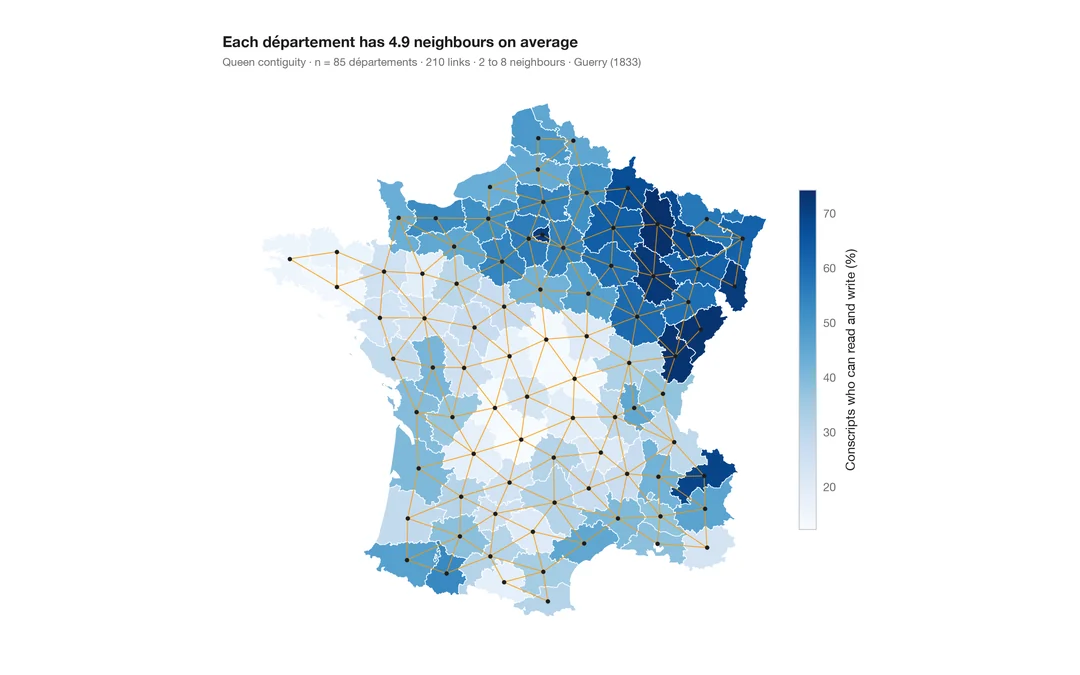
Choropleth with spatial weights
A map of one variable with the neighbour network drawn on top — the structure every spatial statistic relies on.
spdep::poly2nb() + plot(nb, coords)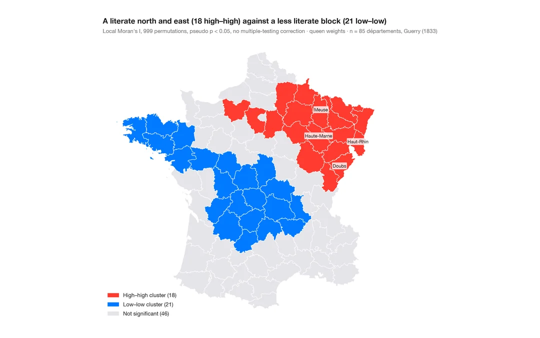
LISA cluster map (local autocorrelation)
Where the clusters and spatial outliers are — local Moran's I for each area, mapped with its permutation significance.
spdep::localmoran_perm() / rgeoda::local_moran()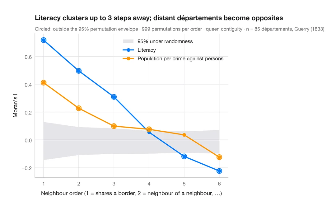
Spatial correlogram
Moran's I at increasing neighbour orders, with a permutation envelope — how far spatial clustering reaches.
spdep::sp.correlogram(method = "I")