LISA cluster map (local autocorrelation)
Where the clusters and spatial outliers are — local Moran's I for each area, mapped with its permutation significance.
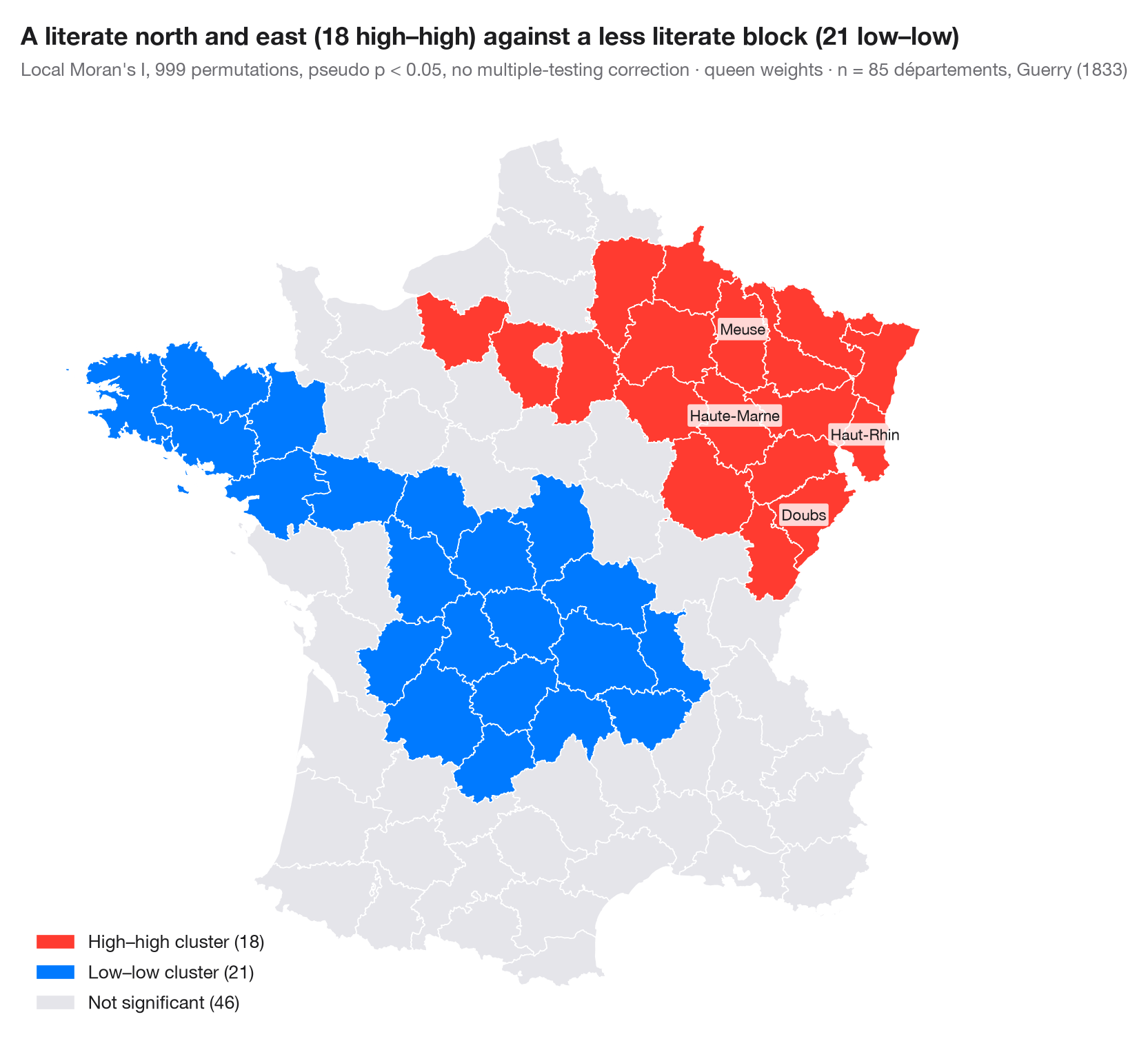
A global statistic says whether a map is clustered; a local indicator of spatial association (LISA; Anselin, 1995) says where. Local Moran's I is computed for each area from its own value and its neighbours' values. Areas whose local statistic is significant (pseudo p < 0.05, 999 conditional permutations) are coloured by quadrant of the Moran scatterplot: high–high and low–low clusters, and high–low or low–high spatial outliers. Everything else is grey.
Two cautions come with every LISA map. The 85 tests are not independent and
are not corrected for multiple comparisons, so a few significant areas are
expected by chance alone; and a significant area marks the core of a
cluster, which usually extends to its neighbours. Data are Guerry's (1833)
literacy rates for 85 départements, loaded with libpysal; the statistic
comes from esda.Moran_Local and the map from GeoPandas.
import geopandas as gpd
import matplotlib.pyplot as plt
import numpy as np
from esda.moran import Moran_Local
from libpysal import examples, weights
from matplotlib.patches import Patch

# Data: literacy of military conscripts in 85 départements, c. 1830 (Guerry, 1833)
g = gpd.read_file(examples.load_example("Guerry").get_path("guerry.shp"))
y = g["Litercy"].to_numpy(dtype=float)

w = weights.Queen.from_dataframe(g, use_index=False)
w.transform = "r"
lisa = Moran_Local(y, w, permutations=999, seed=1)

# Quadrants: 1 high–high, 2 low–high, 3 low–low, 4 high–low; grey if not significant
labels = {1: "High–high cluster", 3: "Low–low cluster", 2: "Low–high outlier", 4: "High–low outlier"}
colors = {1: "#FF3B30", 3: "#007AFF", 2: "#9FCBFF", 4: "#FFA8A2"}
sig = lisa.p_sim < 0.05
g["cluster"] = np.where(sig, lisa.q, 0)
counts = {k: int((g["cluster"] == k).sum()) for k in labels}

fig, ax = plt.subplots(figsize=(8, 7.4))
g.plot(color=[colors.get(c, "#E5E5EA") for c in g["cluster"]], edgecolor="white", linewidth=0.6, ax=ax)
handles = [Patch(color=colors[k], label=f"{labels[k]} ({counts[k]})") for k in labels if counts[k]]
handles.append(Patch(color="#E5E5EA", label=f"Not significant ({int((~sig).sum())})"))
ax.legend(handles=handles, loc="lower left", fontsize=9.5)
ax.set_axis_off()

# Name the strongest cluster cores
for _, r in g.assign(p=lisa.p_sim, Is=lisa.Is)[sig].nlargest(4, "Is").iterrows():
    c = r.geometry.representative_point()
    ax.annotate(r["Dprtmnt"], (c.x, c.y), fontsize=8, ha="center", color="#1D1D1F",
                bbox=dict(boxstyle="round,pad=0.15", fc="white", ec="none", alpha=0.8))

north = g.centroid.y[g["cluster"] == 1].mean() > g.centroid.y[g["cluster"] == 3].mean()
where = "north and east" if north else "south"
ax.set_title(f"A literate {where} ({counts[1]} high–high) against a less literate "
             f"block ({counts[3]} low–low)", pad=26)
ax.text(0, 1.02, f"Local Moran's I, 999 permutations, pseudo p < 0.05, no multiple-testing correction · "
        f"queen weights · n = {w.n} départements, Guerry (1833)",
        transform=ax.transAxes, fontsize=9.5, color="#6E6E73")
plt.show()
Figures use the optional PyStatlas style: add plt.style.use("pystatlas.mplstyle") to match the look exactly.
Data source
- Guerry's moral statistics of France, c. 1830 (85 départements). Guerry, A.-M. (1833). Essai sur la statistique morale de la France. Crochard. Data as compiled in Friendly, M. (2007). A.-M. Guerry's moral statistics of France: Challenges for multivariable spatial analysis. Statistical Science, 22(3), 368–399. https://doi.org/10.1214/07-STS241
Prepared by the Center for Spatial Data Science (University of Chicago) from the R package Guerry (Friendly and Dray), provided “as is”. Fetched once and cached by libpysal (examples.load_example("Guerry")). Variables come from Guerry's tables as translated by Whitt and Reinking (2002).
The examples illustrate statistical methods. Their titles describe what each figure shows in these particular data — often a small, dated or partial sample — not the author's position on the substantive question. For interpretation, context and data quality, rely on the original sources cited here.
How to cite
PyStatlas is created and maintained by Thierry Warin. If it helped your work, please cite it.
Warin, T. (2026). LISA cluster map (local autocorrelation). In PyStatlas: A Python Gallery of Statistical Graphics for the Social Sciences. https://warint.github.io/pystatlas/spatial-data/lisa-cluster-map/
@misc{warin2026statlas,
  author       = {Warin, Thierry},
  title        = {PyStatlas: A Python Gallery of Statistical Graphics for the Social Sciences},
  year         = {2026},
  howpublished = {\url{https://warint.github.io/pystatlas/}},
  note         = {Source code: https://github.com/warint/pystatlas}
}More in Spatial data
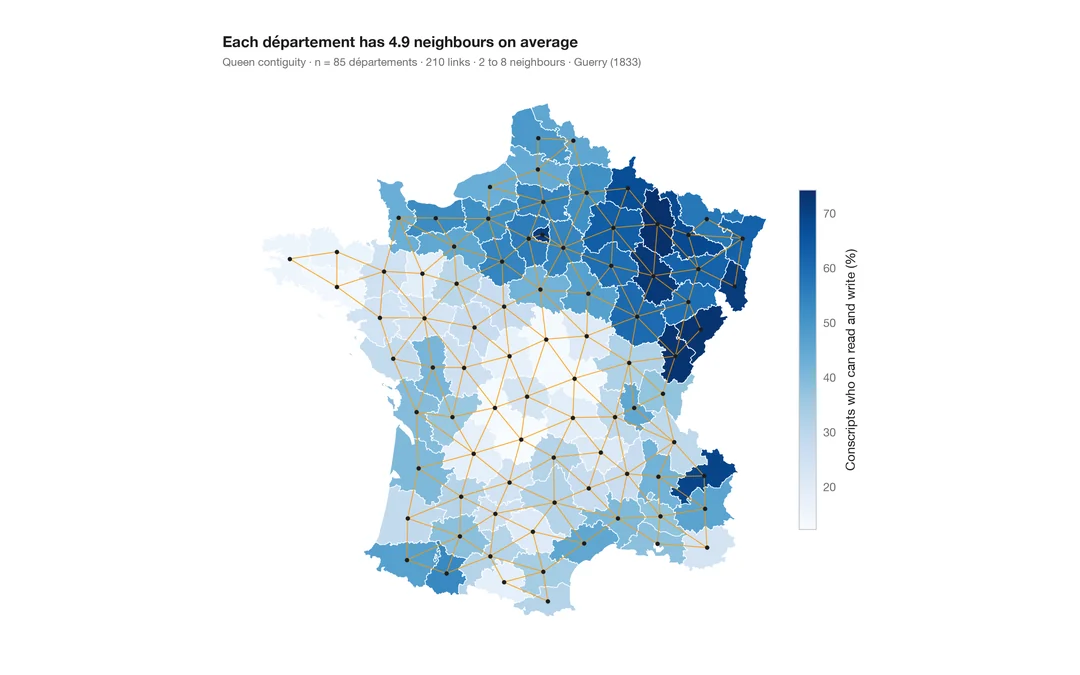
Choropleth with spatial weights
A map of one variable with the neighbour network drawn on top — the structure every spatial statistic relies on.
spdep::poly2nb() + plot(nb, coords)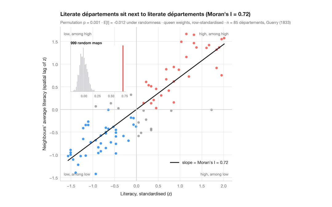
Moran scatterplot (global autocorrelation)
Each area against the average of its neighbours, with Moran's I, its permutation test and the reference distribution.
spdep::moran.plot() + spdep::moran.mc()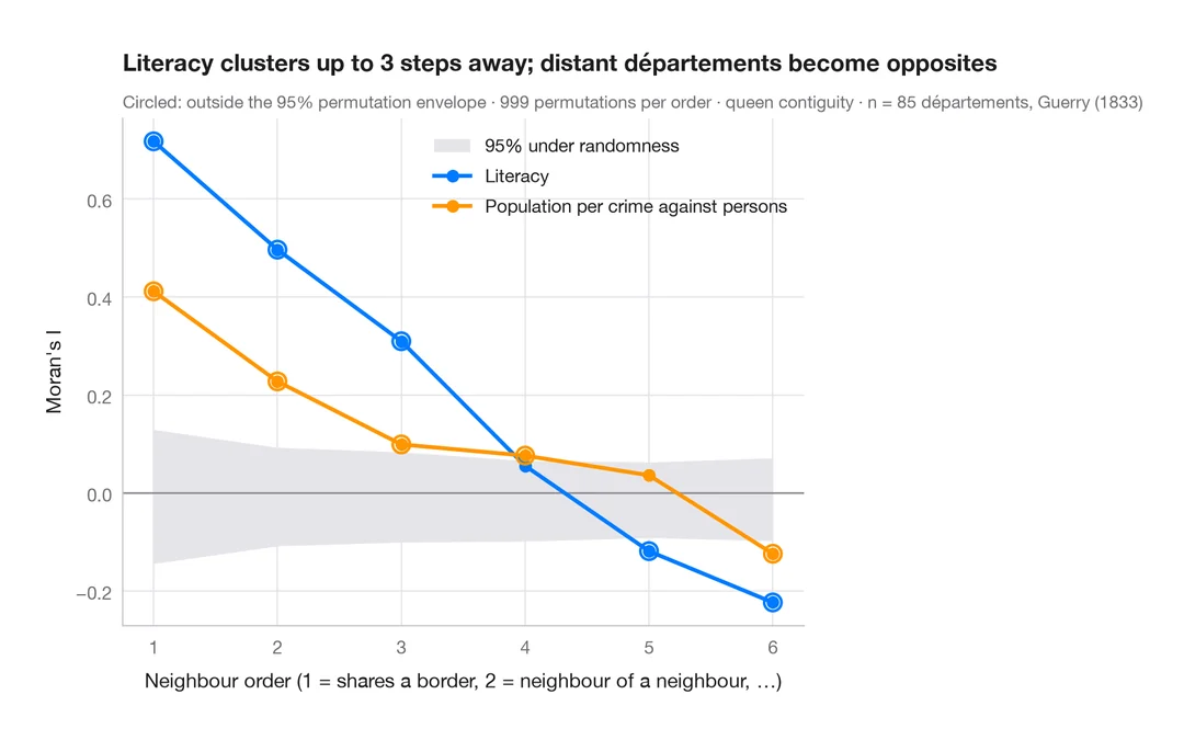
Spatial correlogram
Moran's I at increasing neighbour orders, with a permutation envelope — how far spatial clustering reaches.
spdep::sp.correlogram(method = "I")