莫兰散点图(全局自相关)
每个地区与其邻居平均值的对比,附莫兰 I、置换检验及参照分布。
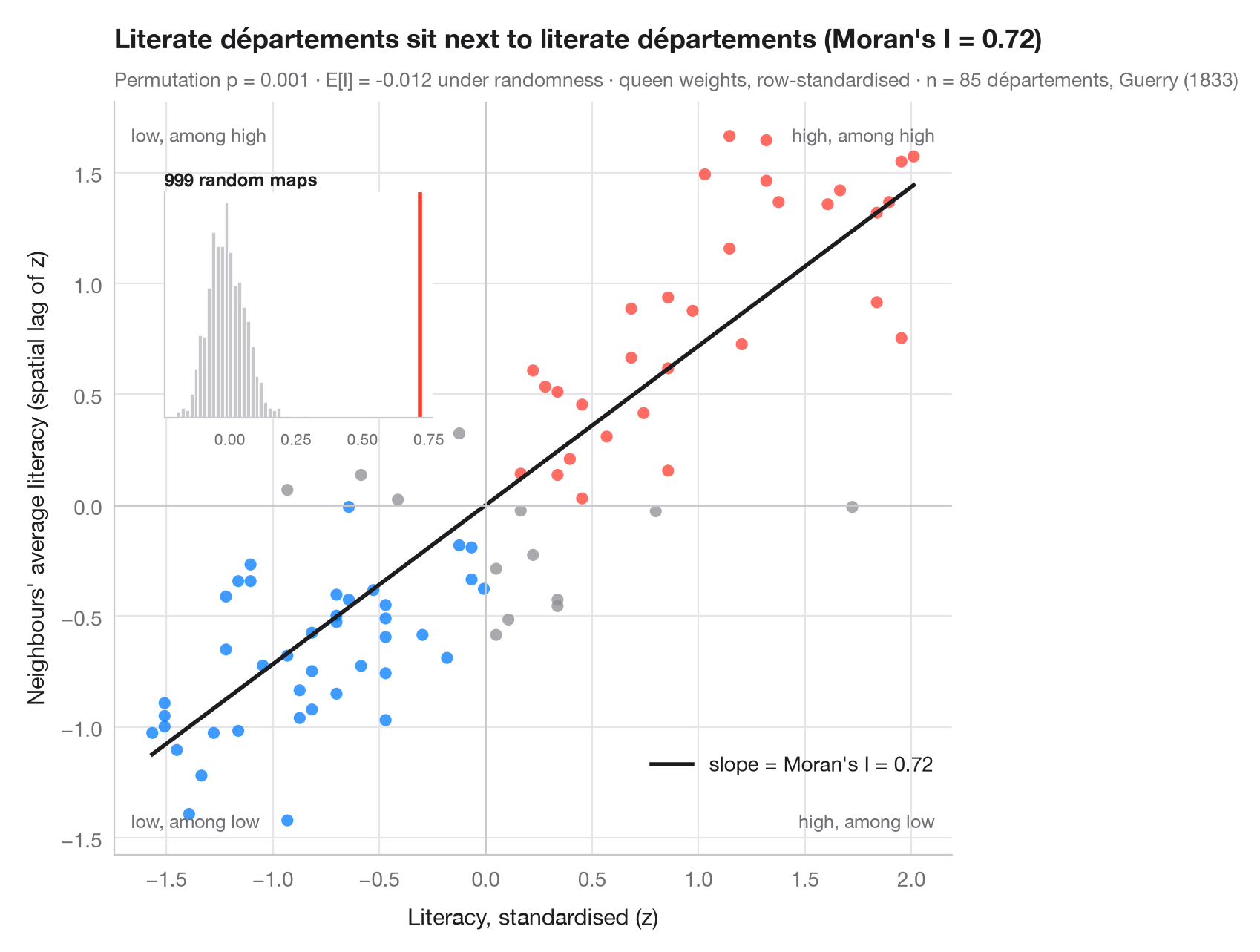
全局空间自相关针对整张地图提出一个问题:相似的数值是否比偶然情况下更常相邻?莫兰散点图以图形方式回答。每个点是一个地区:横轴为其自身(标准化后的)数值,纵轴为其邻居的平均值——即空间滞后。使用行标准化权重时,拟合直线的斜率恰好就是莫兰 I(Moran, 1950)。右上和左下象限的点是与邻居相似的地区;另外两个象限是空间异常值。
推断通过置换完成:将数值在地图上随机打乱 999 次,每次重新计算 I。插图展示了空间随机性下的参照分布;伪 p 值是至少与观测 I 同样极端的置换所占比例。数据为盖里(1833 年)85 个省的识字率,用 libpysal 加载;权重为后式邻接,统计量来自 esda.Moran。
代码及图中文字均为英文。
import geopandas as gpd
import matplotlib.pyplot as plt
import numpy as np
from esda.moran import Moran
from libpysal import examples, weights

# Data: literacy of military conscripts in 85 départements, c. 1830 (Guerry, 1833)
g = gpd.read_file(examples.load_example("Guerry").get_path("guerry.shp"))
y = g["Litercy"].to_numpy(dtype=float)

# Row-standardised queen weights, Moran's I with 999 permutations
w = weights.Queen.from_dataframe(g, use_index=False)
w.transform = "r"
mi = Moran(y, w, permutations=999)
z = (y - y.mean()) / y.std()
lag = weights.lag_spatial(w, z)              # average of the neighbours' z-scores

fig, ax = plt.subplots(figsize=(8, 6.2))
quad = np.select([(z > 0) & (lag > 0), (z < 0) & (lag < 0)], ["#FF3B30", "#007AFF"], "#8E8E93")
ax.scatter(z, lag, s=34, c=quad, alpha=0.75, lw=0)
xs = np.array([z.min(), z.max()])
ax.plot(xs, mi.I * xs, color="#1D1D1F", lw=2, label=f"slope = Moran's I = {mi.I:.2f}")
ax.axhline(0, color="#C7C7CC", lw=1); ax.axvline(0, color="#C7C7CC", lw=1)
for (tx, ty, txt) in [(0.98, 0.97, "high, among high"), (0.02, 0.03, "low, among low"),
                      (0.02, 0.97, "low, among high"), (0.98, 0.03, "high, among low")]:
    ax.text(tx, ty, txt, transform=ax.transAxes, ha="right" if tx > 0.5 else "left",
            va="top" if ty > 0.5 else "bottom", fontsize=9, color="#6E6E73")
ax.set_xlabel("Literacy, standardised (z)")
ax.set_ylabel("Neighbours' average literacy (spatial lag of z)")
ax.grid(axis="x")
ax.legend(loc="lower right", bbox_to_anchor=(1, 0.08))

# Inset: reference distribution of I under spatial randomness
ins = ax.inset_axes([0.06, 0.58, 0.32, 0.3])
ins.hist(mi.sim, bins=30, color="#C7C7CC", edgecolor="white")
ins.axvline(mi.I, color="#FF3B30", lw=2)
ins.set_title("999 random maps", fontsize=8.5, loc="left", pad=3)
ins.tick_params(labelsize=7.5); ins.set_yticks([]); ins.grid(False)

ax.set_title(f"Literate départements sit next to literate départements (Moran's I = {mi.I:.2f})", pad=26)
ax.text(0, 1.02, f"Permutation p = {mi.p_sim:.3f} · E[I] = {mi.EI:.3f} under randomness · "
        f"queen weights, row-standardised · n = {w.n} départements, Guerry (1833)",
        transform=ax.transAxes, fontsize=9.5, color="#6E6E73")
plt.show()
图表使用了可选的 PyStatlas 样式:添加 plt.style.use("pystatlas.mplstyle") 即可完全还原其外观。
数据来源
- Guerry's moral statistics of France, c. 1830 (85 départements). Guerry, A.-M. (1833). Essai sur la statistique morale de la France. Crochard. Data as compiled in Friendly, M. (2007). A.-M. Guerry's moral statistics of France: Challenges for multivariable spatial analysis. Statistical Science, 22(3), 368–399. https://doi.org/10.1214/07-STS241
Prepared by the Center for Spatial Data Science (University of Chicago) from the R package Guerry (Friendly and Dray), provided “as is”. Fetched once and cached by libpysal (examples.load_example("Guerry")). Variables come from Guerry's tables as translated by Whitt and Reinking (2002).
这些示例用于说明统计方法。图表标题描述的是该图在这些特定数据中呈现的内容——这些数据往往样本较小、年代较早或并不完整——而不是作者对实质问题的立场。关于解释、背景和数据质量,请以此处引用的原始来源为准。
如何引用
PyStatlas 由 Thierry Warin 创建并维护。如果它对你的工作有所帮助,敬请引用。
Warin, T. (2026). Moran scatterplot (global autocorrelation). In PyStatlas: A Python Gallery of Statistical Graphics for the Social Sciences. https://warint.github.io/pystatlas/spatial-data/moran-scatterplot/
@misc{warin2026statlas,
  author       = {Warin, Thierry},
  title        = {PyStatlas: A Python Gallery of Statistical Graphics for the Social Sciences},
  year         = {2026},
  howpublished = {\url{https://warint.github.io/pystatlas/}},
  note         = {Source code: https://github.com/warint/pystatlas}
}