Moran scatterplot (global autocorrelation) — PyStatlas: A Python Gallery of Statistical Graphics for the Social Sciences

Warin, Thierry

モラン散布図（大域的自己相関）

各地域をその近隣の平均と比べ、モランの I、並べ替え検定、参照分布を添えます。

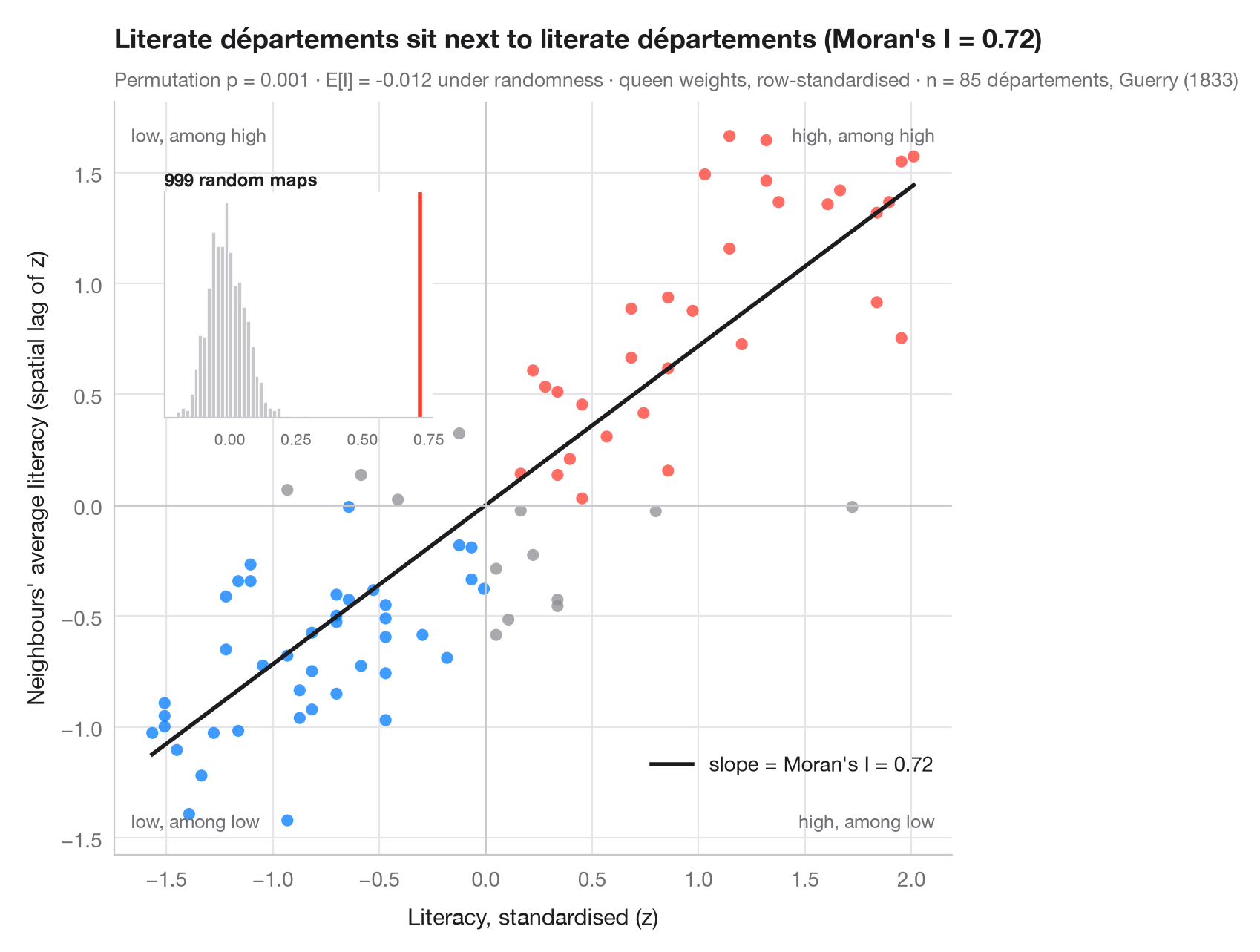
大域的な空間自己相関は、地図全体について 1 つの問いを立てます。似た値どうしが、偶然で説明できる以上に隣り合っているか。モラン散布図はこれを視覚的に答えます。各点は地域で、横軸はその地域自身の（標準化した）値、縦軸は近隣の平均、すなわち空間ラグです。行標準化した重みを使うと、当てはめた直線の傾きはちょうどモランの I（Moran, 1950）になります。右上と左下の象限の点は近隣に似た地域、残りの 2 つの象限には空間的な外れ値が入ります。

推測は並べ替えで行います。値を地図上で 999 回無作為に入れ替え、そのたびに I を計算し直します。挿入図は空間的無作為性のもとでの参照分布で、擬似 p 値は観測された I 以上に極端な入れ替えの割合です。データはゲリー（1833 年）の 85 県の識字率で、libpysal で読み込み、重みはクイーン型隣接、統計量は esda.Moran によります。

コードおよび図中のテキストは英語です。

moran-scatterplot.py · 44 行

ダウンロード GitHub

import geopandas as gpd
import matplotlib.pyplot as plt
import numpy as np
from esda.moran import Moran
from libpysal import examples, weights

# Data: literacy of military conscripts in 85 départements, c. 1830 (Guerry, 1833)
g = gpd.read_file(examples.load_example("Guerry").get_path("guerry.shp"))
y = g["Litercy"].to_numpy(dtype=float)

# Row-standardised queen weights, Moran's I with 999 permutations
w = weights.Queen.from_dataframe(g, use_index=False)
w.transform = "r"
mi = Moran(y, w, permutations=999)
z = (y - y.mean()) / y.std()
lag = weights.lag_spatial(w, z)              # average of the neighbours' z-scores

fig, ax = plt.subplots(figsize=(8, 6.2))
quad = np.select([(z > 0) & (lag > 0), (z < 0) & (lag < 0)], ["#FF3B30", "#007AFF"], "#8E8E93")
ax.scatter(z, lag, s=34, c=quad, alpha=0.75, lw=0)
xs = np.array([z.min(), z.max()])
ax.plot(xs, mi.I * xs, color="#1D1D1F", lw=2, label=f"slope = Moran's I = {mi.I:.2f}")
ax.axhline(0, color="#C7C7CC", lw=1); ax.axvline(0, color="#C7C7CC", lw=1)
for (tx, ty, txt) in [(0.98, 0.97, "high, among high"), (0.02, 0.03, "low, among low"),
                      (0.02, 0.97, "low, among high"), (0.98, 0.03, "high, among low")]:
    ax.text(tx, ty, txt, transform=ax.transAxes, ha="right" if tx > 0.5 else "left",
            va="top" if ty > 0.5 else "bottom", fontsize=9, color="#6E6E73")
ax.set_xlabel("Literacy, standardised (z)")
ax.set_ylabel("Neighbours' average literacy (spatial lag of z)")
ax.grid(axis="x")
ax.legend(loc="lower right", bbox_to_anchor=(1, 0.08))

# Inset: reference distribution of I under spatial randomness
ins = ax.inset_axes([0.06, 0.58, 0.32, 0.3])
ins.hist(mi.sim, bins=30, color="#C7C7CC", edgecolor="white")
ins.axvline(mi.I, color="#FF3B30", lw=2)
ins.set_title("999 random maps", fontsize=8.5, loc="left", pad=3)
ins.tick_params(labelsize=7.5); ins.set_yticks([]); ins.grid(False)

ax.set_title(f"Literate départements sit next to literate départements (Moran's I = {mi.I:.2f})", pad=26)
ax.text(0, 1.02, f"Permutation p = {mi.p_sim:.3f} · E[I] = {mi.EI:.3f} under randomness · "
        f"queen weights, row-standardised · n = {w.n} départements, Guerry (1833)",
        transform=ax.transAxes, fontsize=9.5, color="#6E6E73")
plt.show()

図にはオプションの PyStatlas スタイルを使用しています。同じ見た目にするには plt.style.use("pystatlas.mplstyle") を追加してください。

データの出典

Guerry's moral statistics of France, c. 1830 (85 départements). Guerry, A.-M. (1833). Essai sur la statistique morale de la France. Crochard. Data as compiled in Friendly, M. (2007). A.-M. Guerry's moral statistics of France: Challenges for multivariable spatial analysis. Statistical Science, 22(3), 368–399. https://doi.org/10.1214/07-STS241
Prepared by the Center for Spatial Data Science (University of Chicago) from the R package Guerry (Friendly and Dray), provided “as is”. Fetched once and cached by libpysal (examples.load_example("Guerry")). Variables come from Guerry's tables as translated by Whitt and Reinking (2002).

これらの例は統計手法を説明するためのものです。図のタイトルは、この特定のデータ（多くは小規模で、古く、部分的な標本）で図が示す内容を述べたものであり、実質的な問いに対する著者の立場ではありません。解釈、背景、データの質については、ここに挙げた元の出典を参照してください。

引用方法

PyStatlas は Thierry Warin が作成・運営しています。研究や業務に役立った場合は、ぜひ引用してください。

Warin, T. (2026). Moran scatterplot (global autocorrelation). In PyStatlas: A Python Gallery of Statistical Graphics for the Social Sciences. https://warint.github.io/pystatlas/spatial-data/moran-scatterplot/

@misc{warin2026statlas,
  author       = {Warin, Thierry},
  title        = {PyStatlas: A Python Gallery of Statistical Graphics for the Social Sciences},
  year         = {2026},
  howpublished = {\url{https://warint.github.io/pystatlas/}},
  note         = {Source code: https://github.com/warint/pystatlas}
}

空間データのその他のグラフ

空間データ

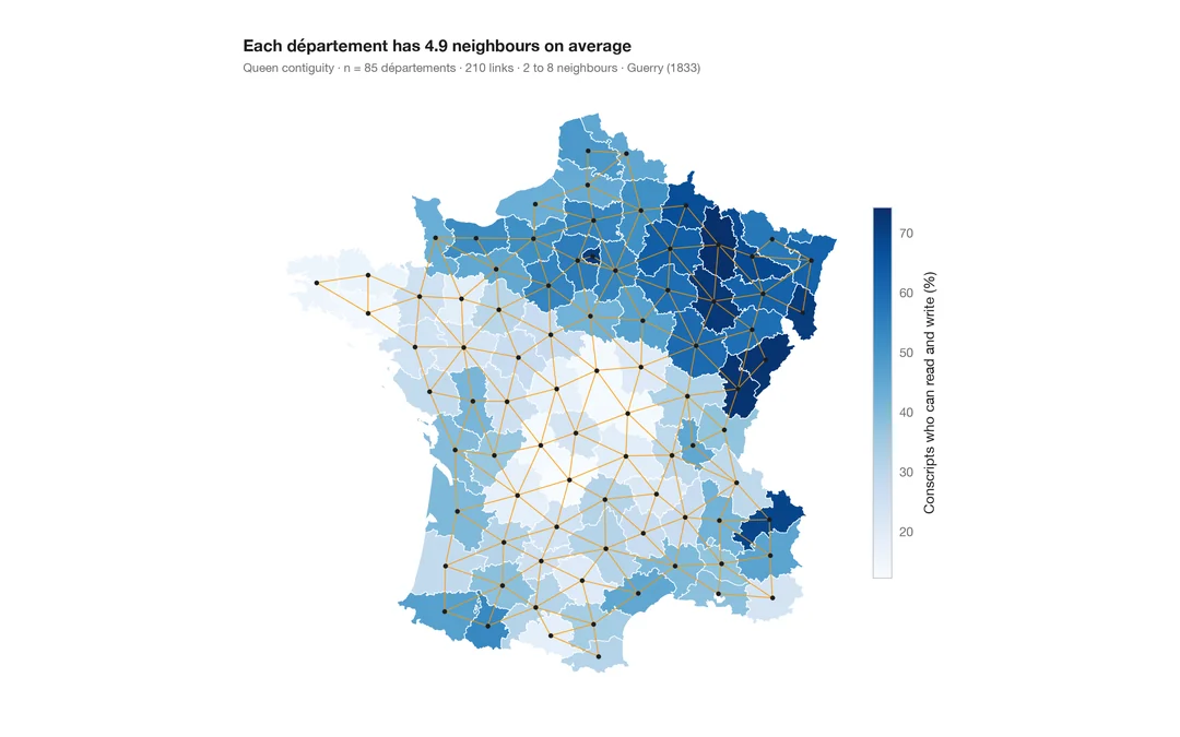
空間重み付きコロプレス図

1 つの変数の地図に近隣ネットワークを重ねた図。あらゆる空間統計の土台となる構造です。

spdep::poly2nb() + plot(nb, coords)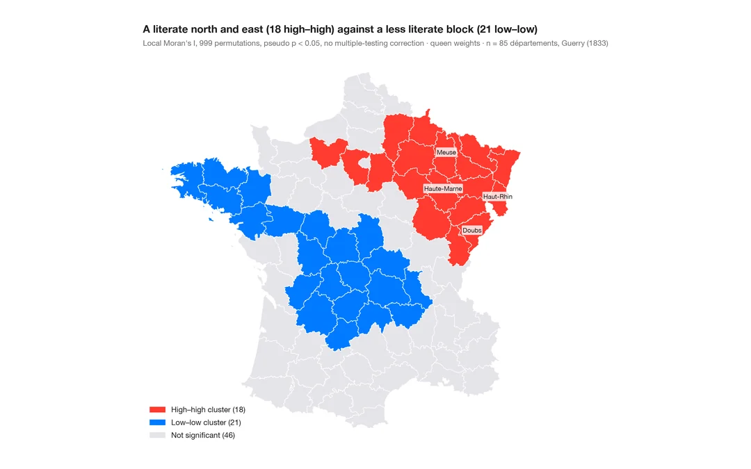

空間データ

LISA クラスター地図（局所的自己相関）

クラスターと空間的外れ値がどこにあるか。各地域の局所モラン I を、並べ替えによる有意性とともに地図に示します。

spdep::localmoran_perm() / rgeoda::local_moran()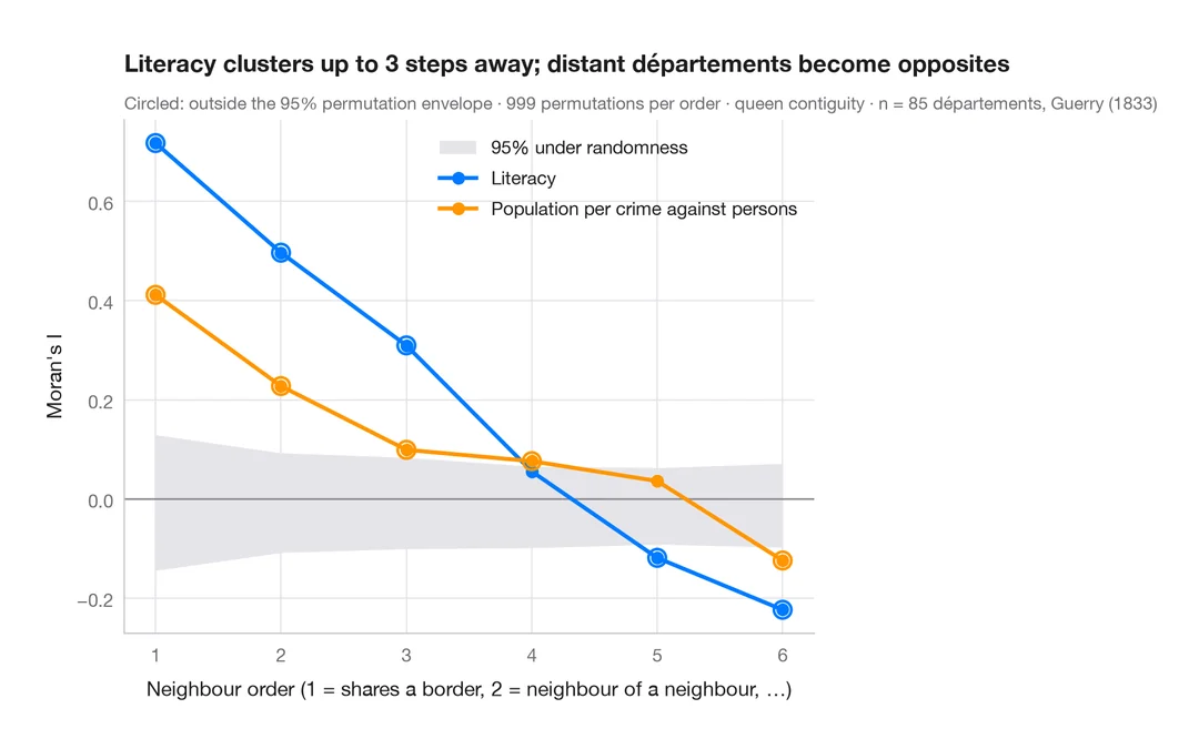

空間データ

空間コレログラム

近隣の次数を広げながらモランの I を求め、並べ替えによる包絡線を添えます。空間的なクラスターがどこまで及ぶかを示します。

spdep::sp.correlogram(method = "I")