空間コレログラム
近隣の次数を広げながらモランの I を求め、並べ替えによる包絡線を添えます。空間的なクラスターがどこまで及ぶかを示します。
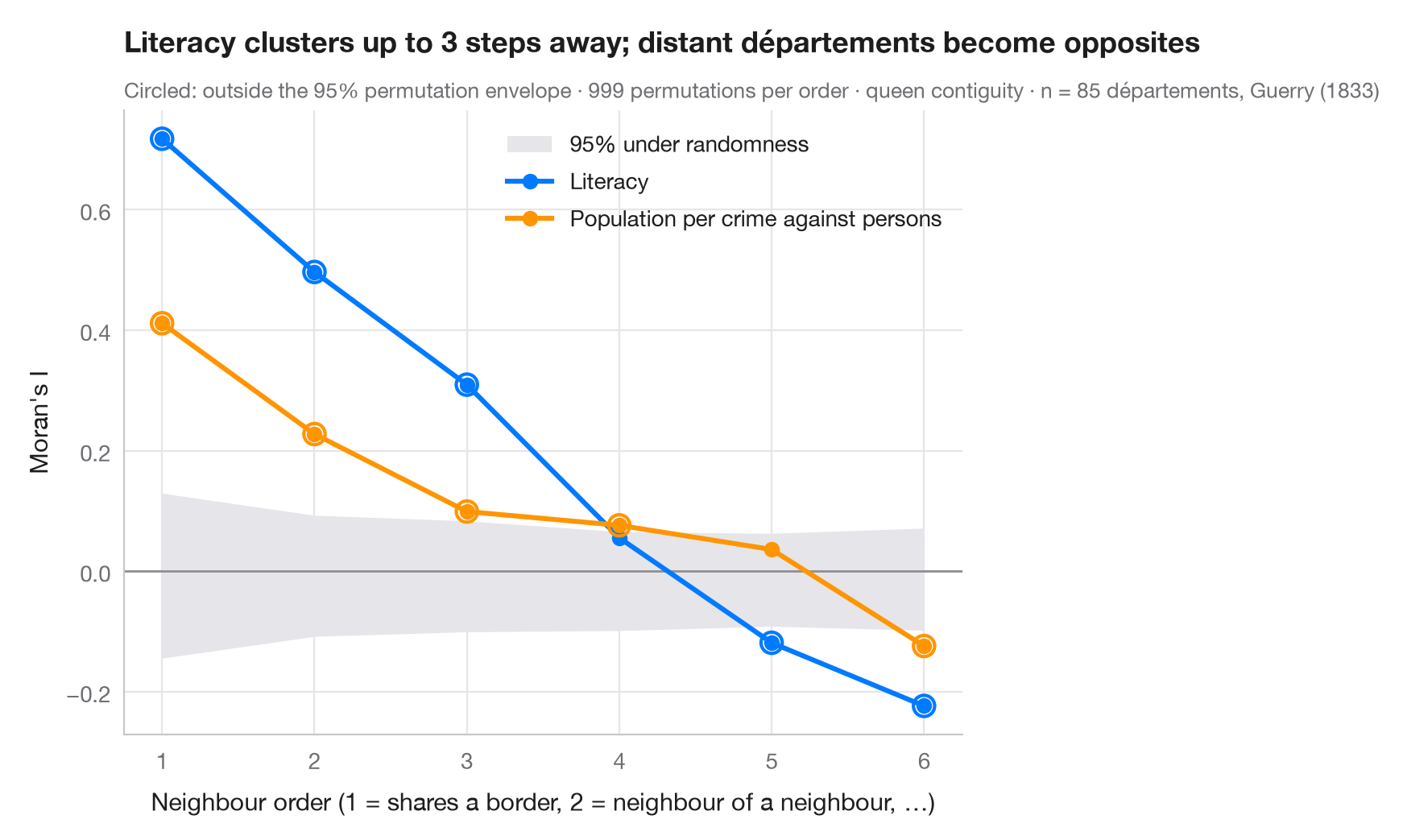
1 次の近隣で計算したモランの I は、最も短い範囲でのクラスター化を測ります。空間コレログラムは、同じ計算を 2 次の近隣(近隣の近隣で、より近いものを除く)、3 次と繰り返します。曲線は現象の空間スケールを示します。何ステップ離れても 2 つの地域は似ているのか、そして遠い地域どうしは正反対(負の I)になるのか。国が 2 つの大きな地域に分かれているときにはそうなります。これは時系列の自己相関関数の空間版です。
灰色の帯は、各次数で 999 回の並べ替えから求めた、空間的無作為性のもとでの I の 95% 範囲で、帯の外の点は空間構造がなければ起こりにくいものです。ゲリー(1833 年)の道徳統計から 85 県の 2 つの変数を比べています。識字率と、対人犯罪 1 件あたりの人口(高いほど犯罪が少ない)です。重みは libpysal.weights.higher_order による高次のクイーン型隣接を行標準化したもので、I は esda.Moran によります。
コードおよび図中のテキストは英語です。
import geopandas as gpd
import matplotlib.pyplot as plt
import numpy as np
from esda.moran import Moran
from libpysal import examples, weights

# Data: 85 French départements, c. 1830 (Guerry, 1833)
g = gpd.read_file(examples.load_example("Guerry").get_path("guerry.shp"))
variables = {"Litercy": ("Literacy", "#007AFF"),
             "Crm_prs": ("Population per crime against persons", "#FF9500")}

w1 = weights.Queen.from_dataframe(g, use_index=False)
orders = range(1, 7)
res = {v: [] for v in variables}
for k in orders:
    wk = weights.higher_order(w1, k, silence_warnings=True)    # exactly k steps away
    wk.transform = "r"
    for v in variables:
        m = Moran(g[v].to_numpy(dtype=float), wk, permutations=999)
        res[v].append((m.I, *np.percentile(m.sim, [2.5, 97.5]), m.p_sim))

fig, ax = plt.subplots(figsize=(8, 5))
env = np.array(res["Litercy"])[:, 1:3]                   # envelope (similar for both variables)
ax.fill_between(orders, env[:, 0], env[:, 1], color="#E5E5EA", lw=0, label="95% under randomness")
ax.axhline(0, color="#8E8E93", lw=1)
for v, (name, c) in variables.items():
    a = np.array(res[v])
    ax.plot(orders, a[:, 0], color=c, lw=2.2, marker="o", label=name)
    out = (a[:, 0] < a[:, 1]) | (a[:, 0] > a[:, 2])
    ax.scatter(np.array(orders)[out], a[out, 0], s=90, facecolor="none", edgecolor=c, lw=1.5, zorder=4)
ax.set_xticks(list(orders))
ax.set_xlabel("Neighbour order (1 = shares a border, 2 = neighbour of a neighbour, …)")
ax.set_ylabel("Moran's I")
ax.grid(axis="x")
ax.legend(loc="upper right")

lit = np.array(res["Litercy"])
reach = max(k for k, (I, lo, hi, p) in zip(orders, lit) if I > hi)
ax.set_title(f"Literacy clusters up to {reach} steps away; distant départements become opposites", pad=26)
ax.text(0, 1.02, "Circled: outside the 95% permutation envelope · 999 permutations per order · "
        f"queen contiguity · n = {w1.n} départements, Guerry (1833)",
        transform=ax.transAxes, fontsize=9.5, color="#6E6E73")
plt.show()
図にはオプションの PyStatlas スタイル を使用しています。同じ見た目にするには plt.style.use("pystatlas.mplstyle") を追加してください。
データの出典
- Guerry's moral statistics of France, c. 1830 (85 départements). Guerry, A.-M. (1833). Essai sur la statistique morale de la France. Crochard. Data as compiled in Friendly, M. (2007). A.-M. Guerry's moral statistics of France: Challenges for multivariable spatial analysis. Statistical Science, 22(3), 368–399. https://doi.org/10.1214/07-STS241
Prepared by the Center for Spatial Data Science (University of Chicago) from the R package Guerry (Friendly and Dray), provided “as is”. Fetched once and cached by libpysal (examples.load_example("Guerry")). Variables come from Guerry's tables as translated by Whitt and Reinking (2002).
これらの例は統計手法を説明するためのものです。図のタイトルは、この特定のデータ(多くは小規模で、古く、部分的な標本)で図が示す内容を述べたものであり、実質的な問いに対する著者の立場ではありません。解釈、背景、データの質については、ここに挙げた元の出典を参照してください。
引用方法
PyStatlas は Thierry Warin が作成・運営しています。研究や業務に役立った場合は、ぜひ引用してください。
Warin, T. (2026). Spatial correlogram. In PyStatlas: A Python Gallery of Statistical Graphics for the Social Sciences. https://warint.github.io/pystatlas/spatial-data/spatial-correlogram/
@misc{warin2026statlas,
  author       = {Warin, Thierry},
  title        = {PyStatlas: A Python Gallery of Statistical Graphics for the Social Sciences},
  year         = {2026},
  howpublished = {\url{https://warint.github.io/pystatlas/}},
  note         = {Source code: https://github.com/warint/pystatlas}
}空間データのその他のグラフ
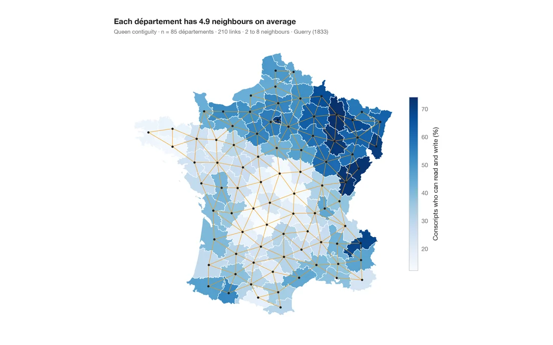
空間重み付きコロプレス図
1 つの変数の地図に近隣ネットワークを重ねた図。あらゆる空間統計の土台となる構造です。
spdep::poly2nb() + plot(nb, coords)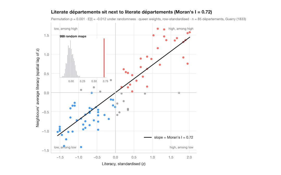
モラン散布図(大域的自己相関)
各地域をその近隣の平均と比べ、モランの I、並べ替え検定、参照分布を添えます。
spdep::moran.plot() + spdep::moran.mc()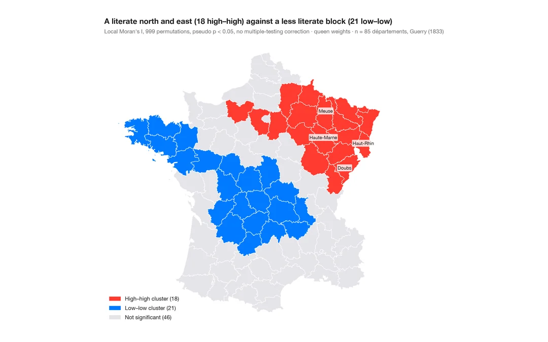
LISA クラスター地図(局所的自己相関)
クラスターと空間的外れ値がどこにあるか。各地域の局所モラン I を、並べ替えによる有意性とともに地図に示します。
spdep::localmoran_perm() / rgeoda::local_moran()