空間重み付きコロプレス図
1 つの変数の地図に近隣ネットワークを重ねた図。あらゆる空間統計の土台となる構造です。
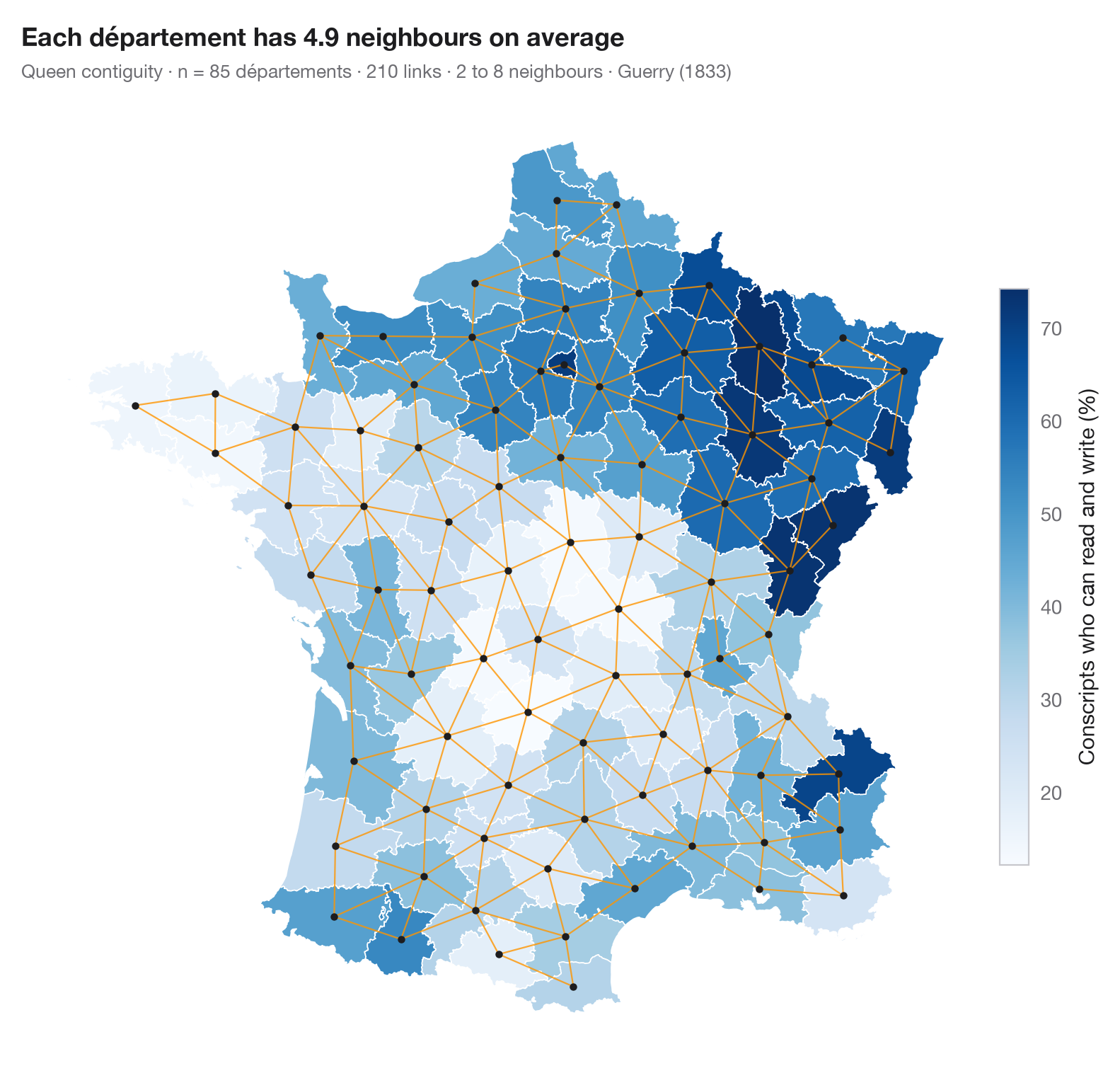
すべての空間統計は、どの地域とどの地域を近隣とみなすかを決めるところから始まります。この図は、検定を行う前にその決定を見せます。1 つの変数のコロプレス図に、近隣どうしの地域の中心を結ぶ線を重ねています。ここでは境界または角を共有する地域を近隣とし(クイーン型隣接)、重み行列の各行はのちに標準化されるため、ある地域の「空間ラグ」は近隣の平均になります。ルーク型隣接、k 近傍、距離帯など別の選び方をすれば別のネットワークになり、結果も変わりうるので、ネットワークは確認する価値があります。
データはアンドレ=ミシェル・ゲリーの『フランスの道徳統計に関する試論』(1833 年)で、1830 年頃の 85 県を、Center for Spatial Data Science が整備したものを libpysal(examples.load_example("Guerry")、初回のみ取得しその後は保存)で読み込んでいます。変数は読み書きのできる徴集兵の割合です。重みは libpysal.weights.Queen、地図は GeoPandas で描いています。
コードおよび図中のテキストは英語です。
import geopandas as gpd
import matplotlib.pyplot as plt
import numpy as np
from libpysal import examples, weights

# Data: 85 French départements, c. 1830 (Guerry, 1833)
g = gpd.read_file(examples.load_example("Guerry").get_path("guerry.shp"))
y = g["Litercy"]                      # % of conscripts who can read and write

# Queen contiguity: neighbours share a border or a corner
w = weights.Queen.from_dataframe(g, use_index=False)
cards = np.array(list(w.cardinalities.values()))
xy = np.column_stack([g.centroid.x, g.centroid.y])

fig, ax = plt.subplots(figsize=(8, 7.4))
g.plot(column=y, cmap="Blues", edgecolor="white", linewidth=0.6, ax=ax, legend=True,
       legend_kwds=dict(label="Conscripts who can read and write (%)", shrink=0.6, pad=0.01))
for i, nbrs in w.neighbors.items():
    for j in nbrs:
        if i < j:                      # draw each link once
            ax.plot(*xy[[i, j]].T, color="#FF9500", lw=0.8, alpha=0.8)
ax.scatter(*xy.T, s=10, color="#1D1D1F", zorder=3)
ax.set_axis_off()
ax.set_title(f"Each département has {w.mean_neighbors:.1f} neighbours on average", pad=26)
ax.text(0, 1.02, f"Queen contiguity · n = {w.n} départements · {int(w.s0 / 2)} links · "
        f"{cards.min()} to {cards.max()} neighbours · Guerry (1833)",
        transform=ax.transAxes, fontsize=9.5, color="#6E6E73")
plt.show()
図にはオプションの PyStatlas スタイル を使用しています。同じ見た目にするには plt.style.use("pystatlas.mplstyle") を追加してください。
データの出典
- Guerry's moral statistics of France, c. 1830 (85 départements). Guerry, A.-M. (1833). Essai sur la statistique morale de la France. Crochard. Data as compiled in Friendly, M. (2007). A.-M. Guerry's moral statistics of France: Challenges for multivariable spatial analysis. Statistical Science, 22(3), 368–399. https://doi.org/10.1214/07-STS241
Prepared by the Center for Spatial Data Science (University of Chicago) from the R package Guerry (Friendly and Dray), provided “as is”. Fetched once and cached by libpysal (examples.load_example("Guerry")). Variables come from Guerry's tables as translated by Whitt and Reinking (2002).
これらの例は統計手法を説明するためのものです。図のタイトルは、この特定のデータ(多くは小規模で、古く、部分的な標本)で図が示す内容を述べたものであり、実質的な問いに対する著者の立場ではありません。解釈、背景、データの質については、ここに挙げた元の出典を参照してください。
引用方法
PyStatlas は Thierry Warin が作成・運営しています。研究や業務に役立った場合は、ぜひ引用してください。
Warin, T. (2026). Choropleth with spatial weights. In PyStatlas: A Python Gallery of Statistical Graphics for the Social Sciences. https://warint.github.io/pystatlas/spatial-data/spatial-weights/
@misc{warin2026statlas,
  author       = {Warin, Thierry},
  title        = {PyStatlas: A Python Gallery of Statistical Graphics for the Social Sciences},
  year         = {2026},
  howpublished = {\url{https://warint.github.io/pystatlas/}},
  note         = {Source code: https://github.com/warint/pystatlas}
}空間データのその他のグラフ
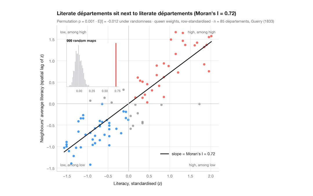
モラン散布図(大域的自己相関)
各地域をその近隣の平均と比べ、モランの I、並べ替え検定、参照分布を添えます。
spdep::moran.plot() + spdep::moran.mc()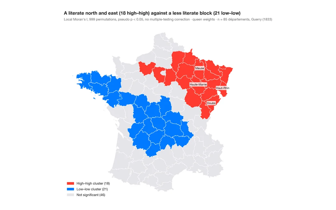
LISA クラスター地図(局所的自己相関)
クラスターと空間的外れ値がどこにあるか。各地域の局所モラン I を、並べ替えによる有意性とともに地図に示します。
spdep::localmoran_perm() / rgeoda::local_moran()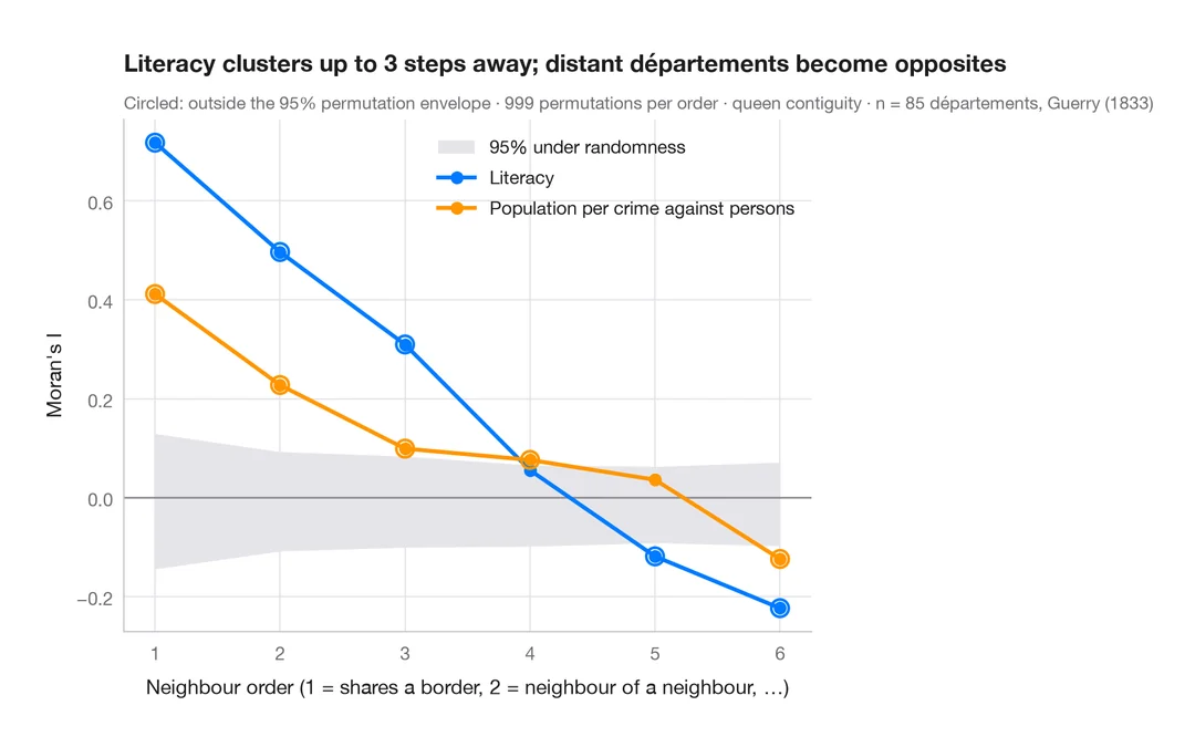
空間コレログラム
近隣の次数を広げながらモランの I を求め、並べ替えによる包絡線を添えます。空間的なクラスターがどこまで及ぶかを示します。
spdep::sp.correlogram(method = "I")