Q–Q plot with confidence band
Normal quantile–quantile plots with a 95% envelope, for a raw and a logged variable.
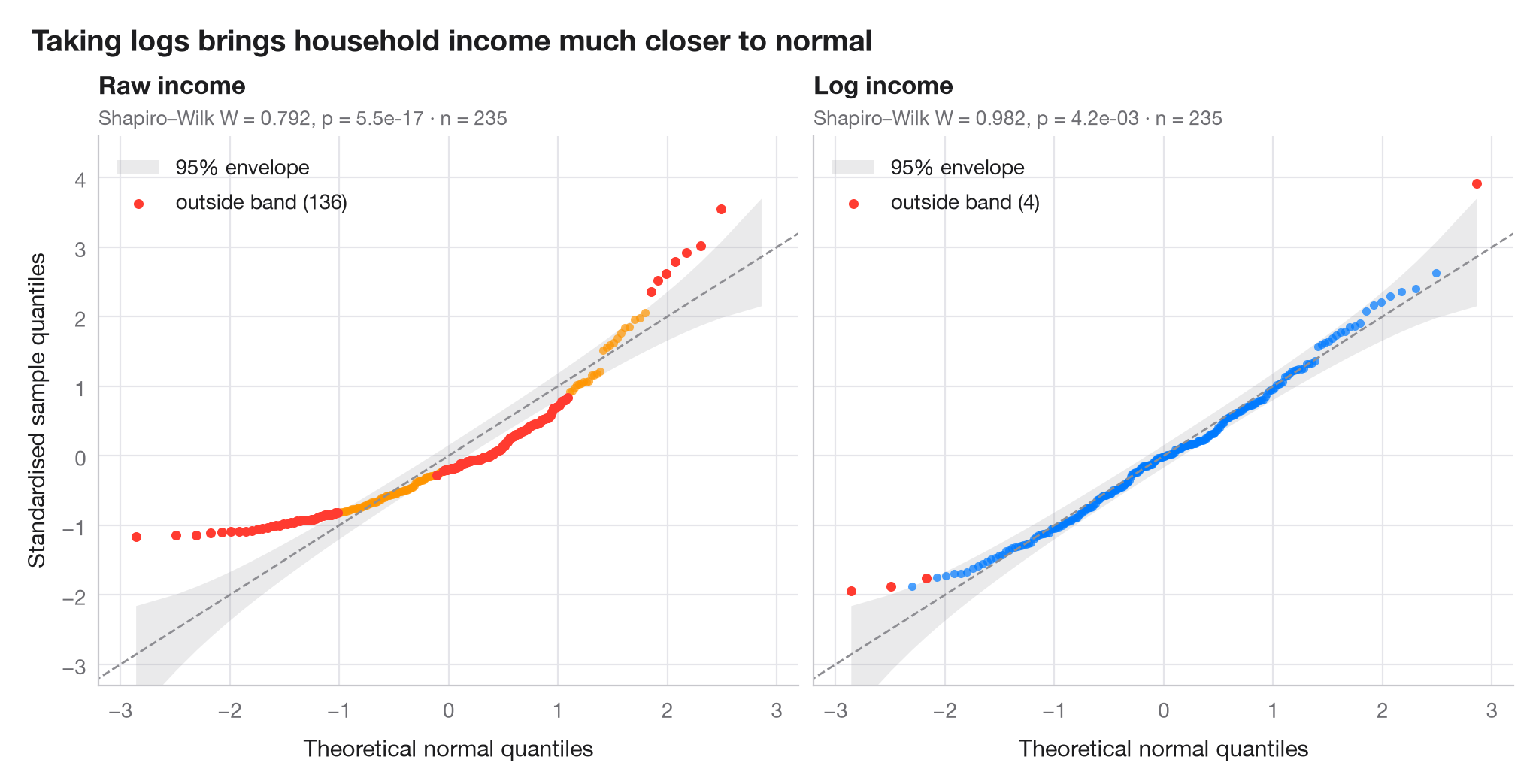
A quantile–quantile plot puts the sorted, standardised data against the quantiles a normal distribution would produce. Normal data fall on the diagonal; a curved, banana-shaped pattern means skewness. The shaded band is a 95% pointwise envelope built from the Beta distribution of normal order statistics, so points outside it are more extreme than chance allows.
Data are household incomes of 235 Belgian working-class families (Engel's
food-expenditure data, bundled with statsmodels). The left panel shows
raw income, the right panel its logarithm. Quantiles come from
scipy.stats.norm.ppf, the envelope from scipy.stats.beta.ppf, and each
panel reports a Shapiro–Wilk test.
import matplotlib.pyplot as plt
import numpy as np
import statsmodels.api as sm
from scipy import stats

# Data: household income, raw and log-transformed
income = sm.datasets.engel.load_pandas().data["income"].to_numpy()
samples = {"Raw income": income, "Log income": np.log(income)}
palette = ["#FF9500", "#007AFF"]

fig, axes = plt.subplots(1, 2, figsize=(10, 5), sharex=True, sharey=True)
for ax, (name, x), c in zip(axes, samples.items(), palette):
    n = len(x)
    z = np.sort((x - x.mean()) / x.std(ddof=1))      # standardised sample quantiles
    pp = (np.arange(1, n + 1) - 0.5) / n              # plotting positions
    theo = stats.norm.ppf(pp)                         # theoretical normal quantiles

    # 95% pointwise envelope: order statistic i of a uniform sample is Beta(i, n-i+1)
    i = np.arange(1, n + 1)
    lo = stats.norm.ppf(stats.beta.ppf(0.025, i, n - i + 1))
    hi = stats.norm.ppf(stats.beta.ppf(0.975, i, n - i + 1))
    outside = (z < lo) | (z > hi)

    ax.fill_between(theo, lo, hi, color="#8E8E93", alpha=0.18, lw=0, label="95% envelope")
    ax.plot([-3.5, 3.5], [-3.5, 3.5], color="#8E8E93", lw=1, ls="--")
    ax.scatter(theo[~outside], z[~outside], s=16, color=c, alpha=0.7, lw=0)
    ax.scatter(theo[outside], z[outside], s=22, color="#FF3B30", lw=0,
               label=f"outside band ({outside.sum()})")

    W, p = stats.shapiro(x)
    ax.set_title(name, pad=20, fontsize=12)
    ax.text(0, 1.02, f"Shapiro–Wilk W = {W:.3f}, p = {p:.1e} · n = {n}",
            transform=ax.transAxes, fontsize=9.5, color="#6E6E73")
    ax.legend(loc="upper left")
    ax.grid(axis="x")
    ax.set_xlabel("Theoretical normal quantiles")

axes[0].set_ylabel("Standardised sample quantiles")
axes[0].set_xlim(-3.2, 3.2)
axes[0].set_ylim(-3.3, 4.6)
fig.suptitle("Taking logs brings household income much closer to normal",
             x=0.01, ha="left", fontsize=14)
plt.show()
Figures use the optional PyStatlas style: add plt.style.use("pystatlas.mplstyle") to match the look exactly.
Data source
- Engel's Belgian household budgets (235 families). Koenker, R., & Bassett, G. (1982). Robust tests for heteroscedasticity based on regression quantiles. Econometrica, 50(1), 43–61. https://doi.org/10.2307/1912528
Engel's (1857) household budget data as used by Koenker and Bassett and distributed with R's quantreg; in statsmodels as sm.datasets.engel; public domain.
The examples illustrate statistical methods. Their titles describe what each figure shows in these particular data — often a small, dated or partial sample — not the author's position on the substantive question. For interpretation, context and data quality, rely on the original sources cited here.
How to cite
PyStatlas is created and maintained by Thierry Warin. If it helped your work, please cite it.
Warin, T. (2026). Q–Q plot with confidence band. In PyStatlas: A Python Gallery of Statistical Graphics for the Social Sciences. https://warint.github.io/pystatlas/distributions/qq-plot/
@misc{warin2026statlas,
  author       = {Warin, Thierry},
  title        = {PyStatlas: A Python Gallery of Statistical Graphics for the Social Sciences},
  year         = {2026},
  howpublished = {\url{https://warint.github.io/pystatlas/}},
  note         = {Source code: https://github.com/warint/pystatlas}
}More in Distributions
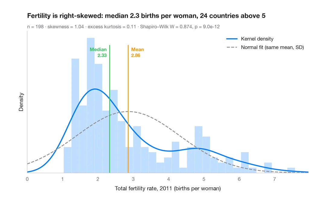
Histogram with density
Histogram, kernel density and fitted normal curve, with shape statistics.
ggplot2::geom_histogram() + geom_density()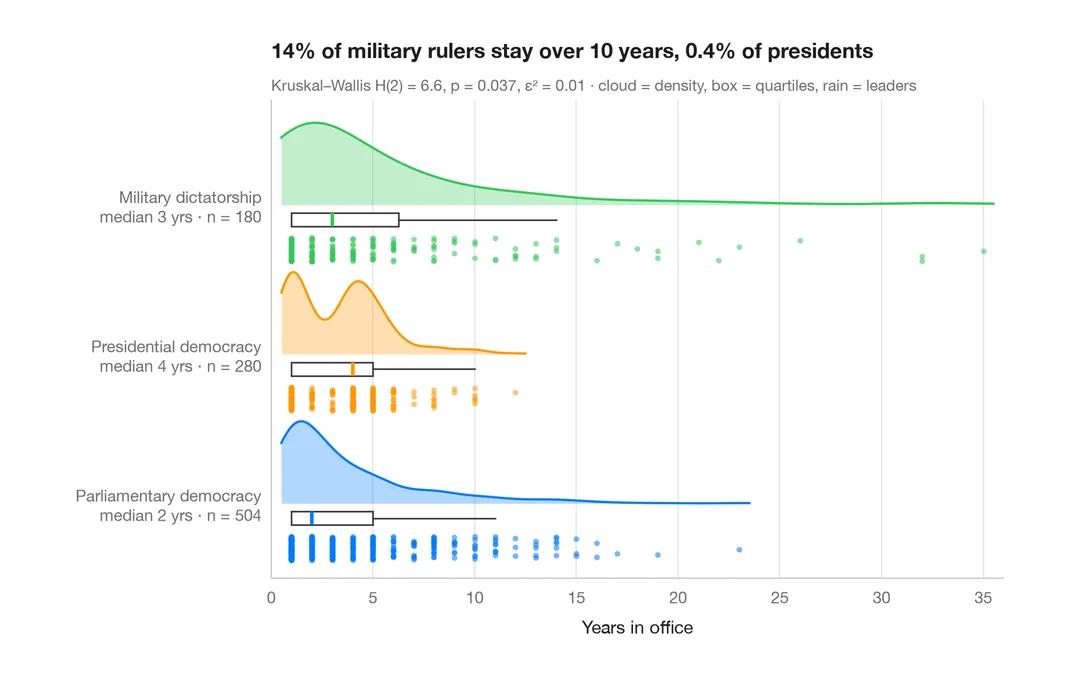
Raincloud plot
Half violin, box plot and raw points per group, drawn horizontally.
ggdist::stat_halfeye() / ggrain::geom_rain()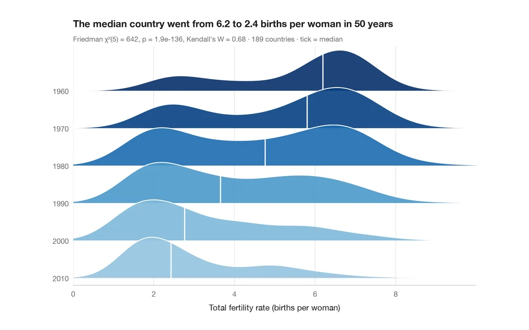
Ridgeline plot
Overlapping density curves to compare one distribution across many groups.
ggridges::geom_density_ridges()