Raincloud plot
Half violin, box plot and raw points per group, drawn horizontally.
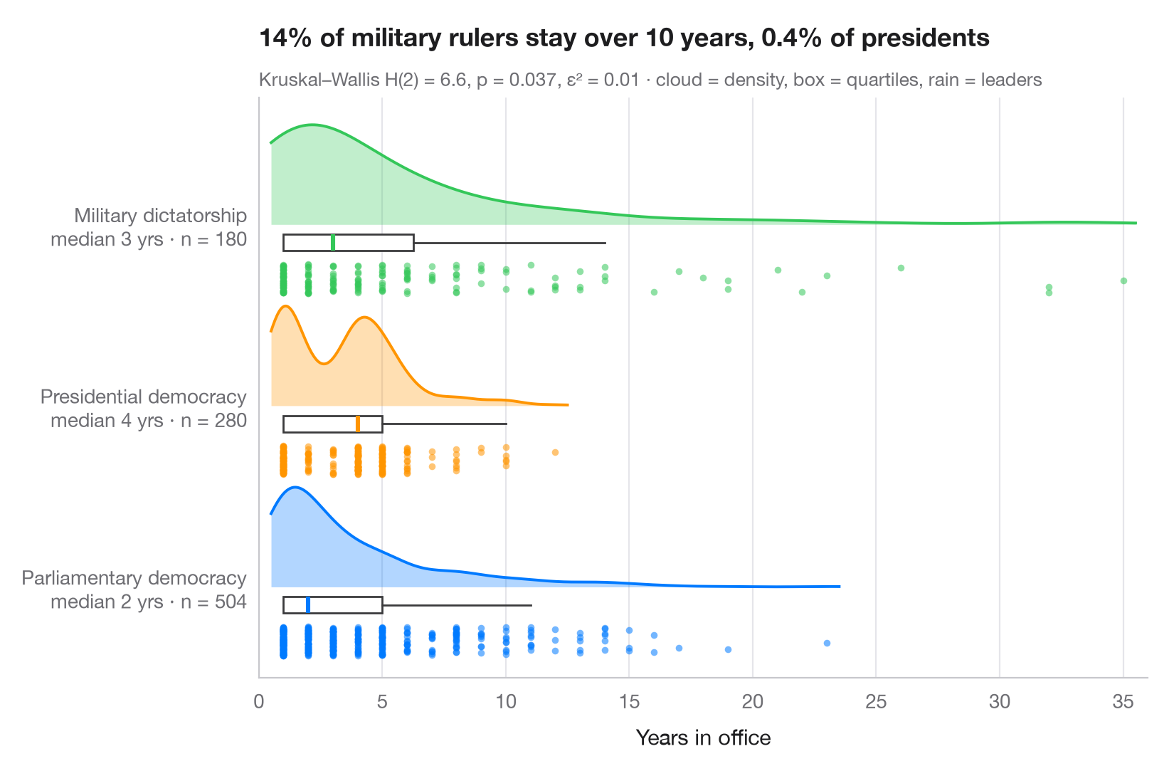
A raincloud plot stacks three views of the same data: a half violin (the "cloud") shows the density, a slim box plot gives the median and quartiles, and the jittered points underneath (the "rain") show every single observation. Nothing is hidden, so bimodality, outliers and small samples are all visible.
Data are the 964 completed spells in office of heads of government between
1946 and 2008 under three regime types, from the Democracy and Dictatorship
data bundled with lifelines (lifelines.datasets.load_dd()); leaders still
in office at the end of the data (censored spells) are left out. The
densities come from scipy.stats.gaussian_kde, and the subtitle reports a
Kruskal–Wallis test (scipy.stats.kruskal) — a rank test, suited to skewed
durations — with ε² as effect size.
import matplotlib.pyplot as plt
import numpy as np
from lifelines.datasets import load_dd
from scipy import stats

# Data: years in office of leaders whose spell ended, by regime type
df = load_dd().query("observed == 1")
groups = {"Parliamentary Dem": "Parliamentary democracy",
          "Presidential Dem": "Presidential democracy", "Military Dict": "Military dictatorship"}
data = [df.loc[df.regime == g, "duration"].to_numpy() for g in groups]
palette = ["#007AFF", "#FF9500", "#34C759"]

# Kruskal–Wallis test + epsilon squared
H, p = stats.kruskal(*data)
n = sum(len(d) for d in data)
eps2 = H / (n - 1)

fig, ax = plt.subplots(figsize=(8, 5.2))
rng = np.random.default_rng(7)
for i, (d, c) in enumerate(zip(data, palette)):
    # Cloud: half violin above the baseline, scaled to a fixed height
    grid = np.linspace(d.min() - 0.5, d.max() + 0.5, 300)  # trim the cloud near the data
    dens = stats.gaussian_kde(d)(grid)
    ax.fill_between(grid, i, i + 0.55 * dens / dens.max(), color=c, alpha=0.3, lw=0)
    ax.plot(grid, i + 0.55 * dens / dens.max(), color=c, lw=1.4)
    # Box: median and quartiles just under the cloud
    ax.boxplot(d, positions=[i - 0.1], widths=0.09, vert=False, showfliers=False,
               patch_artist=True, boxprops=dict(facecolor="white", edgecolor="#3A3A3C", lw=1),
               medianprops=dict(color=c, lw=2.2), whiskerprops=dict(color="#3A3A3C"),
               capprops=dict(visible=False))
    # Rain: jittered raw points below the box
    ax.scatter(d, i - 0.3 + rng.uniform(-0.08, 0.08, len(d)),
               s=12, color=c, alpha=0.55, lw=0)

ax.set_yticks(range(len(groups)), [f"{g}\nmedian {np.median(d):.0f} yrs · n = {len(d)}"
                                   for g, d in zip(groups.values(), data)])
ax.set_ylim(-0.5, len(groups) - 0.3)
ax.set_xlim(0, 36)
ax.grid(axis="x"); ax.grid(axis="y", visible=False)
ax.set_xlabel("Years in office")
share = [np.mean(d > 10) for d in data]
ax.set_title(f"{share[2]:.0%} of military rulers stay over 10 years, "
             f"{share[1]:.1%} of presidents", pad=26)
ax.text(0, 1.02, f"Kruskal–Wallis H(2) = {H:.1f}, p = {p:.3f}, ε² = {eps2:.2f} · "
        "cloud = density, box = quartiles, rain = leaders", transform=ax.transAxes,
        fontsize=9.5, color="#6E6E73")
plt.show()
Figures use the optional PyStatlas style: add plt.style.use("pystatlas.mplstyle") to match the look exactly.
Data source
- Democracy and Dictatorship: leader spells, 1946–2008. Cheibub, J. A., Gandhi, J., & Vreeland, J. R. (2010). Democracy and dictatorship revisited. Public Choice, 143(1–2), 67–101. https://doi.org/10.1007/s11127-009-9491-2
202 countries; distributed with lifelines (lifelines.datasets.load_dd).
The examples illustrate statistical methods. Their titles describe what each figure shows in these particular data — often a small, dated or partial sample — not the author's position on the substantive question. For interpretation, context and data quality, rely on the original sources cited here.
How to cite
PyStatlas is created and maintained by Thierry Warin. If it helped your work, please cite it.
Warin, T. (2026). Raincloud plot. In PyStatlas: A Python Gallery of Statistical Graphics for the Social Sciences. https://warint.github.io/pystatlas/distributions/raincloud/
@misc{warin2026statlas,
  author       = {Warin, Thierry},
  title        = {PyStatlas: A Python Gallery of Statistical Graphics for the Social Sciences},
  year         = {2026},
  howpublished = {\url{https://warint.github.io/pystatlas/}},
  note         = {Source code: https://github.com/warint/pystatlas}
}More in Distributions
Histogram with density
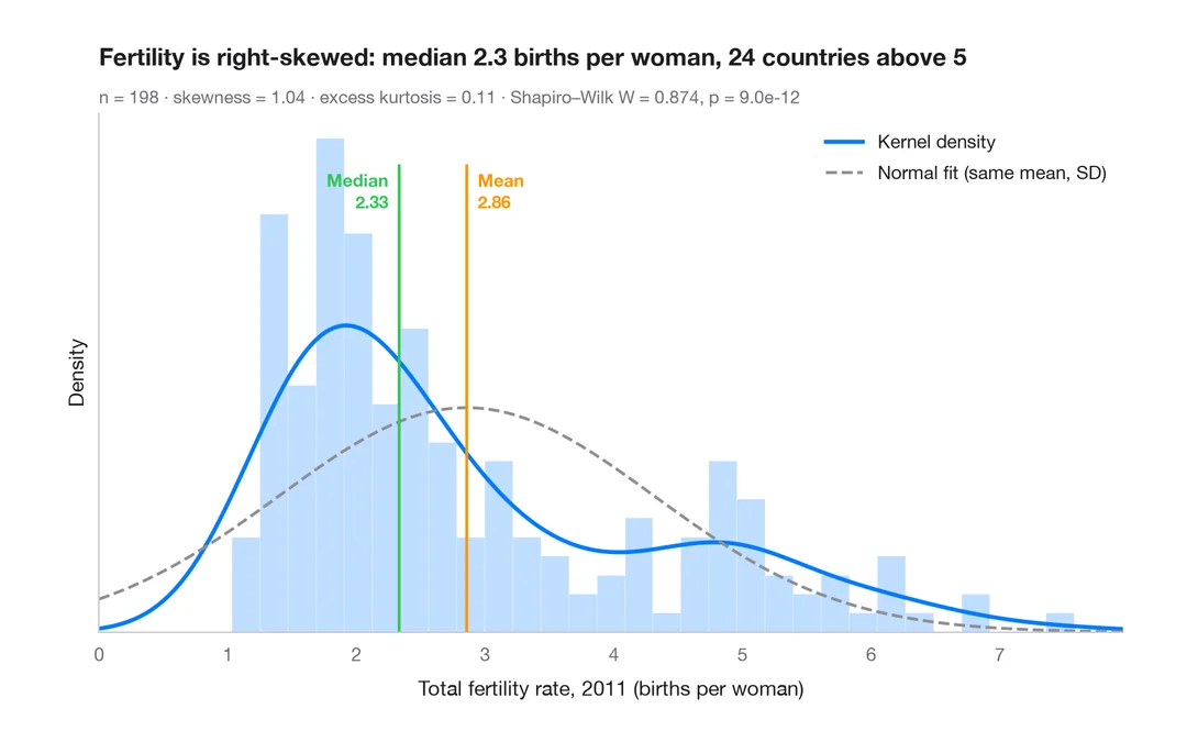
Histogram, kernel density and fitted normal curve, with shape statistics.
ggplot2::geom_histogram() + geom_density()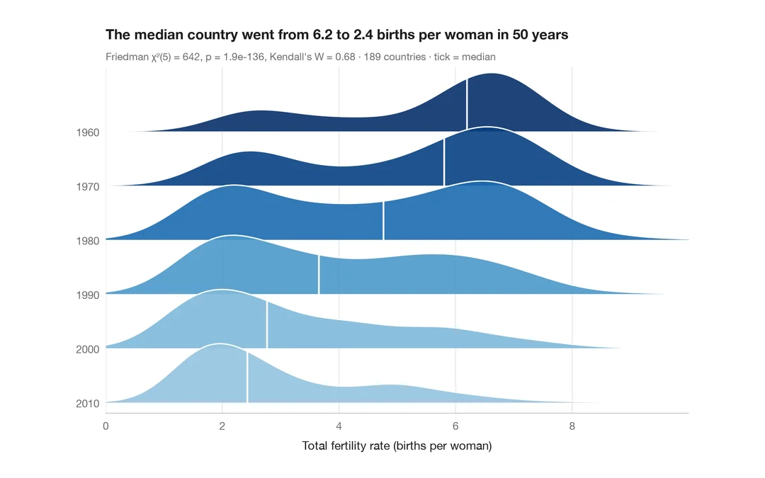
Ridgeline plot
Overlapping density curves to compare one distribution across many groups.
ggridges::geom_density_ridges()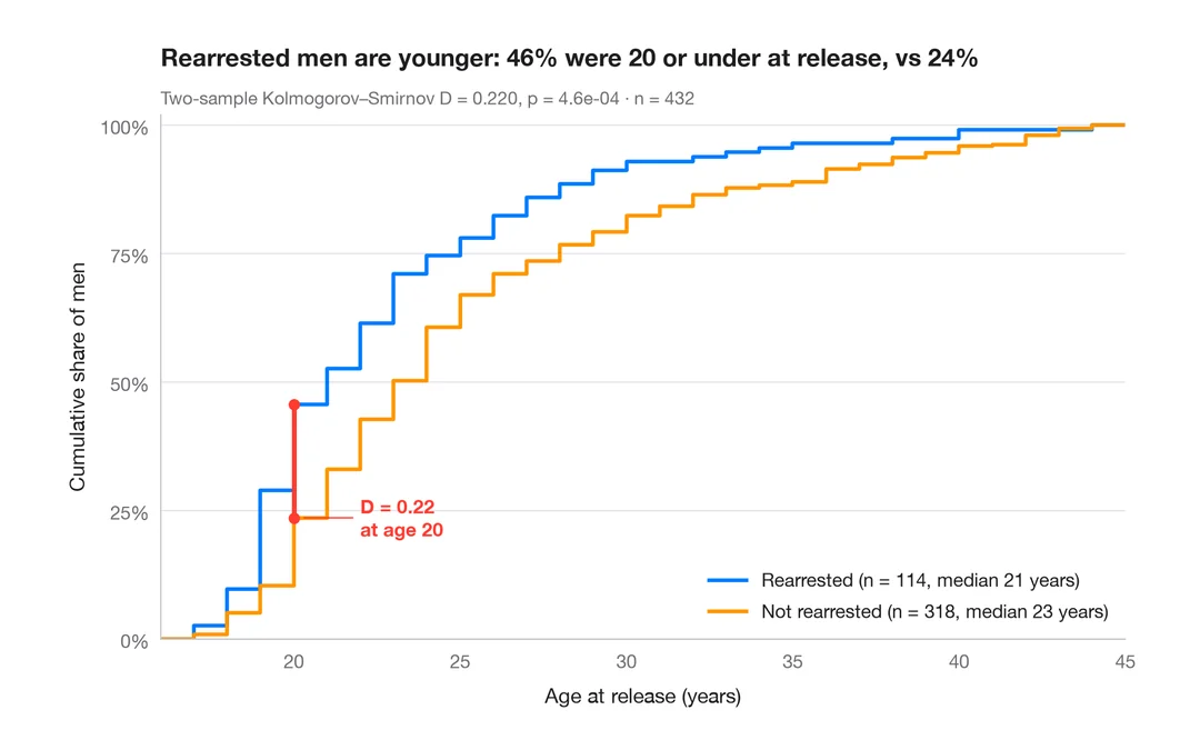
ECDF comparison
Empirical cumulative distributions of two groups, with the Kolmogorov–Smirnov gap.
ggplot2::stat_ecdf()