雨云图
按组横向绘制半边小提琴图、箱线图和原始数据点。
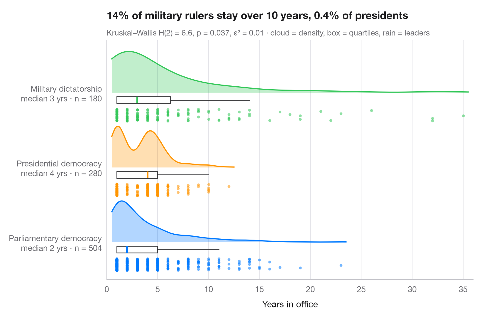
雨云图将同一数据的三种视图叠在一起:半边小提琴图(“云”)展示密度,细长的箱线图给出中位数和四分位数,下方抖动的散点(“雨”)则呈现每一个观测值。没有任何信息被隐藏,因此双峰、离群值和小样本都一目了然。
数据为 1946 年至 2008 年间三种政体下政府首脑已结束的 964 段任期,取自 lifelines 附带的 Democracy and Dictatorship 数据(lifelines.datasets.load_dd());数据截止时仍在任的领导人(删失任期)未纳入。密度由 scipy.stats.gaussian_kde 计算,副标题报告 Kruskal–Wallis 检验(scipy.stats.kruskal)——一种适用于偏态时长数据的秩检验——并以 ε² 作为效应量。
代码及图中文字均为英文。
import matplotlib.pyplot as plt
import numpy as np
from lifelines.datasets import load_dd
from scipy import stats

# Data: years in office of leaders whose spell ended, by regime type
df = load_dd().query("observed == 1")
groups = {"Parliamentary Dem": "Parliamentary democracy",
          "Presidential Dem": "Presidential democracy", "Military Dict": "Military dictatorship"}
data = [df.loc[df.regime == g, "duration"].to_numpy() for g in groups]
palette = ["#007AFF", "#FF9500", "#34C759"]

# Kruskal–Wallis test + epsilon squared
H, p = stats.kruskal(*data)
n = sum(len(d) for d in data)
eps2 = H / (n - 1)

fig, ax = plt.subplots(figsize=(8, 5.2))
rng = np.random.default_rng(7)
for i, (d, c) in enumerate(zip(data, palette)):
    # Cloud: half violin above the baseline, scaled to a fixed height
    grid = np.linspace(d.min() - 0.5, d.max() + 0.5, 300)  # trim the cloud near the data
    dens = stats.gaussian_kde(d)(grid)
    ax.fill_between(grid, i, i + 0.55 * dens / dens.max(), color=c, alpha=0.3, lw=0)
    ax.plot(grid, i + 0.55 * dens / dens.max(), color=c, lw=1.4)
    # Box: median and quartiles just under the cloud
    ax.boxplot(d, positions=[i - 0.1], widths=0.09, vert=False, showfliers=False,
               patch_artist=True, boxprops=dict(facecolor="white", edgecolor="#3A3A3C", lw=1),
               medianprops=dict(color=c, lw=2.2), whiskerprops=dict(color="#3A3A3C"),
               capprops=dict(visible=False))
    # Rain: jittered raw points below the box
    ax.scatter(d, i - 0.3 + rng.uniform(-0.08, 0.08, len(d)),
               s=12, color=c, alpha=0.55, lw=0)

ax.set_yticks(range(len(groups)), [f"{g}\nmedian {np.median(d):.0f} yrs · n = {len(d)}"
                                   for g, d in zip(groups.values(), data)])
ax.set_ylim(-0.5, len(groups) - 0.3)
ax.set_xlim(0, 36)
ax.grid(axis="x"); ax.grid(axis="y", visible=False)
ax.set_xlabel("Years in office")
share = [np.mean(d > 10) for d in data]
ax.set_title(f"{share[2]:.0%} of military rulers stay over 10 years, "
             f"{share[1]:.1%} of presidents", pad=26)
ax.text(0, 1.02, f"Kruskal–Wallis H(2) = {H:.1f}, p = {p:.3f}, ε² = {eps2:.2f} · "
        "cloud = density, box = quartiles, rain = leaders", transform=ax.transAxes,
        fontsize=9.5, color="#6E6E73")
plt.show()
图表使用了可选的 PyStatlas 样式:添加 plt.style.use("pystatlas.mplstyle") 即可完全还原其外观。
数据来源
- Democracy and Dictatorship: leader spells, 1946–2008. Cheibub, J. A., Gandhi, J., & Vreeland, J. R. (2010). Democracy and dictatorship revisited. Public Choice, 143(1–2), 67–101. https://doi.org/10.1007/s11127-009-9491-2
202 countries; distributed with lifelines (lifelines.datasets.load_dd).
这些示例用于说明统计方法。图表标题描述的是该图在这些特定数据中呈现的内容——这些数据往往样本较小、年代较早或并不完整——而不是作者对实质问题的立场。关于解释、背景和数据质量,请以此处引用的原始来源为准。
如何引用
PyStatlas 由 Thierry Warin 创建并维护。如果它对你的工作有所帮助,敬请引用。
Warin, T. (2026). Raincloud plot. In PyStatlas: A Python Gallery of Statistical Graphics for the Social Sciences. https://warint.github.io/pystatlas/distributions/raincloud/
@misc{warin2026statlas,
  author       = {Warin, Thierry},
  title        = {PyStatlas: A Python Gallery of Statistical Graphics for the Social Sciences},
  year         = {2026},
  howpublished = {\url{https://warint.github.io/pystatlas/}},
  note         = {Source code: https://github.com/warint/pystatlas}
}