山脊图
以相互重叠的密度曲线比较多个组的同一分布。
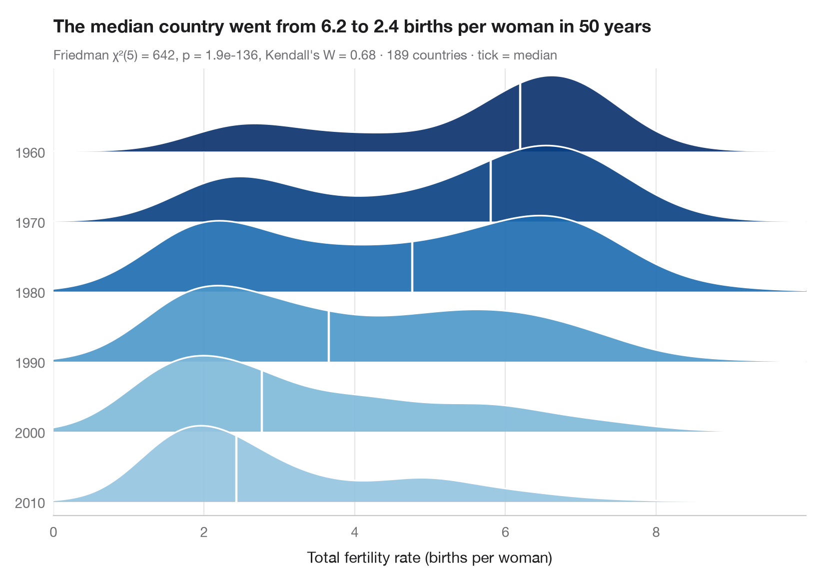
山脊图(又称“joy”图)为每组绘制一条密度曲线并纵向堆叠,曲线之间略有重叠,从而在一张紧凑的图中容纳许多分布。这里每条山脊代表一个年份,从 1960 年到 2010 年每十年一条,展示生育率在世界各国之间的分布;白色刻线标出中位数,颜色也编码中位数(越深表示生育越多),于是人口转变——从高生育率滑向低生育率,其间经历 20 世纪 70、80 年代的双峰世界——一眼即可读出。
数据为 statsmodels 附带的世界银行总和生育率(每名妇女生育的子女数,sm.datasets.fertility),涵盖在 1960、1970、1980、1990、2000 和 2010 年均有数值的 189 个国家(已剔除区域汇总值)。密度由 scipy.stats.gaussian_kde 计算;由于每个国家每年各贡献一个值,副标题报告 Friedman 检验(scipy.stats.friedmanchisquare,以国家为区组),并以 Kendall's W 作为效应量。
代码及图中文字均为英文。
import matplotlib.pyplot as plt
import numpy as np
import statsmodels.api as sm
from scipy import stats

# Data: one row per country, one column per decade (complete cases)
wb = sm.datasets.fertility.load_pandas().data
wb = wb[~wb["Country Name"].str.contains("classification|income levels|members|small states")]  # 5 aggregates
years = ["1960", "1970", "1980", "1990", "2000", "2010"]  # one ridge per decade
tfr = wb[years].dropna()

# Friedman test (countries are blocks) + Kendall's W
chi2, p = stats.friedmanchisquare(*[tfr[m] for m in years])
W = chi2 / (len(tfr) * (len(years) - 1))

grid = np.linspace(0, tfr.values.max() + 1, 400)
medians = tfr.median()
cmap, norm = plt.get_cmap("Blues"), plt.Normalize(medians.min() - 2.5, medians.max())

fig, ax = plt.subplots(figsize=(8, 5.6))
spacing, height = 1.0, 1.8  # vertical gap between ridges, peak height of a ridge
for i, m in enumerate(years):
    base = (len(years) - 1 - i) * spacing  # 1960 on top
    dens = stats.gaussian_kde(tfr[m])(grid)
    curve = base + height * dens / dens.max() * 0.6
    color = cmap(norm(medians[m]))
    ax.fill_between(grid, base, curve, color=color, alpha=0.9, lw=0, zorder=2 * i + 1)
    ax.plot(grid, curve, color="white", lw=1.2, zorder=2 * i + 2)
    ax.axhline(base, color="#C7C7CC", lw=0.6, zorder=2 * i)
    # White tick at the median
    y_med = base + height * stats.gaussian_kde(tfr[m])(medians[m])[0] / dens.max() * 0.6
    ax.plot([medians[m]] * 2, [base, y_med], color="white", lw=1.6, zorder=2 * i + 2)

ax.set_yticks([(len(years) - 1 - i) * spacing for i in range(len(years))], years)
ax.set_ylim(-0.2, (len(years) - 1) * spacing + height * 0.6 + 0.1)
ax.set_xlim(grid[0], grid[-1])
ax.grid(axis="x"); ax.grid(axis="y", visible=False)
ax.spines["left"].set_visible(False)
ax.set_xlabel("Total fertility rate (births per woman)")
ax.set_title(f"The median country went from {medians.iloc[0]:.1f} to {medians.iloc[-1]:.1f} "
             "births per woman in 50 years", pad=26)
ax.text(0, 1.02, f"Friedman χ²({len(years) - 1}) = {chi2:.0f}, p = {p:.1e}, Kendall's W = {W:.2f}"
        f" · {len(tfr)} countries · tick = median", transform=ax.transAxes,
        fontsize=9.5, color="#6E6E73")
plt.show()
图表使用了可选的 PyStatlas 样式:添加 plt.style.use("pystatlas.mplstyle") 即可完全还原其外观。
数据来源
- World Bank fertility rates by country, 1960–2013. World Bank. Fertility rate, total (births per woman), indicator SP.DYN.TFRT.IN. World Development Indicators. https://data.worldbank.org/indicator/SP.DYN.TFRT.IN
Primary sources: UN Population Division, UN Statistical Division, national statistical offices, Eurostat and others. Distributed with statsmodels (sm.datasets.fertility) under the World Bank terms of use.
这些示例用于说明统计方法。图表标题描述的是该图在这些特定数据中呈现的内容——这些数据往往样本较小、年代较早或并不完整——而不是作者对实质问题的立场。关于解释、背景和数据质量,请以此处引用的原始来源为准。
如何引用
PyStatlas 由 Thierry Warin 创建并维护。如果它对你的工作有所帮助,敬请引用。
Warin, T. (2026). Ridgeline plot. In PyStatlas: A Python Gallery of Statistical Graphics for the Social Sciences. https://warint.github.io/pystatlas/distributions/ridgeline/
@misc{warin2026statlas,
  author       = {Warin, Thierry},
  title        = {PyStatlas: A Python Gallery of Statistical Graphics for the Social Sciences},
  year         = {2026},
  howpublished = {\url{https://warint.github.io/pystatlas/}},
  note         = {Source code: https://github.com/warint/pystatlas}
}