リッジラインプロット
重なり合う密度曲線で、多数の群にわたる分布を比較します。
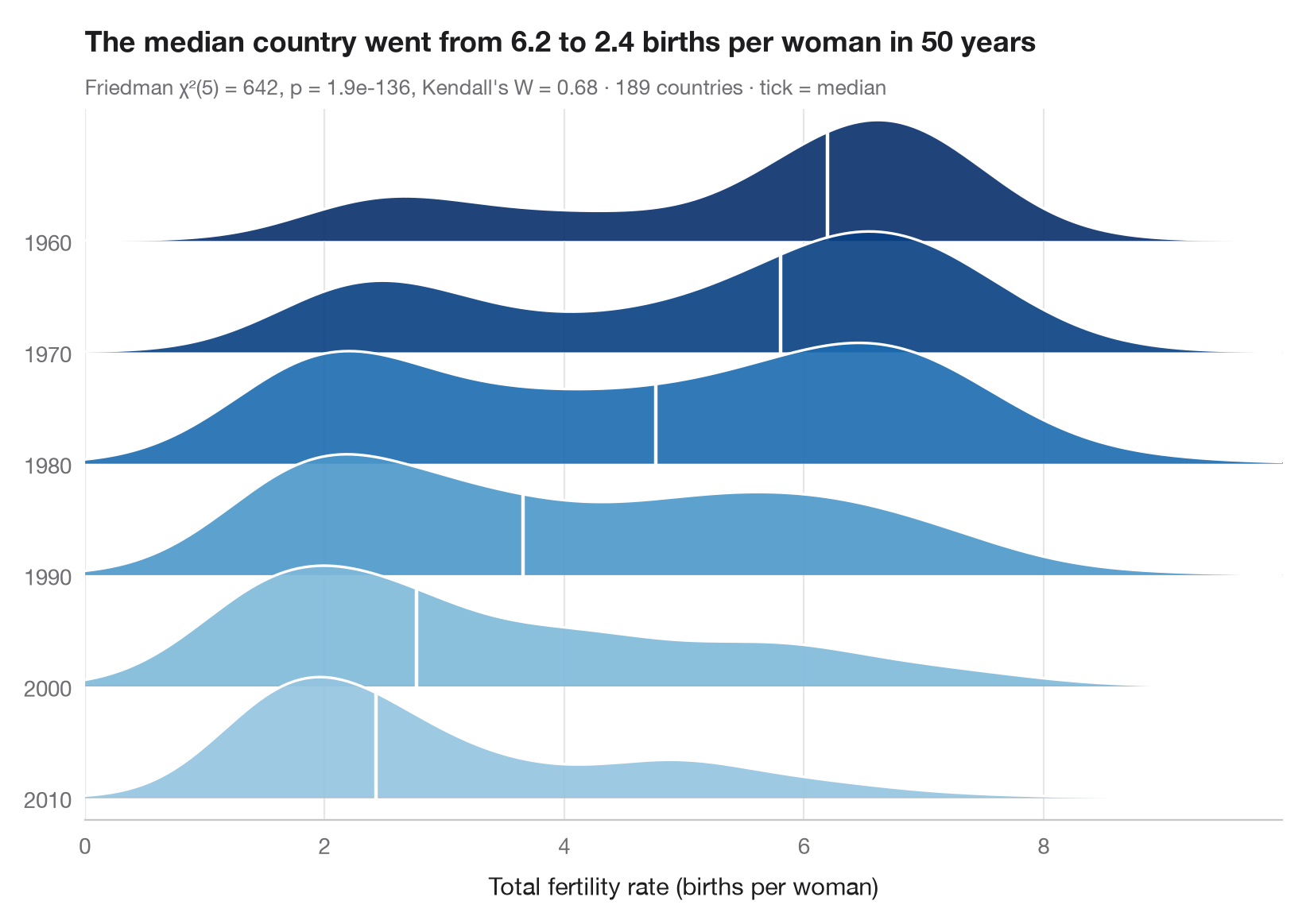
リッジライン(「ジョイ」)プロットは、群ごとの密度曲線を少しずつ重ねて積み上げることで、多数の分布を1枚のコンパクトな図に収めます。ここでは各リッジが1960年から2010年まで10年おきの1年に対応し、世界の国々の間で出生率がどのように分布していたかを表しています。白い目盛りは中央値を示し、色も中央値を表す(濃いほど出生数が多い)ため、人口転換——1970年代と1980年代の二峰型の世界を経て、高出生率から低出生率へと移っていく過程——が一目で読み取れます。
データは statsmodels に同梱されている世界銀行の合計特殊出生率(女性1人あたりの出生数、sm.datasets.fertility)で、1960、1970、1980、1990、2000、2010年のすべてに値がある189か国を対象としています(地域集計値は除外)。密度は scipy.stats.gaussian_kde で求めています。各国が年ごとに1つの値をもつため、サブタイトルには国をブロックとしたフリードマン検定(scipy.stats.friedmanchisquare)の結果を、効果量ケンドールの W とともに示しています。
コードおよび図中のテキストは英語です。
import matplotlib.pyplot as plt
import numpy as np
import statsmodels.api as sm
from scipy import stats

# Data: one row per country, one column per decade (complete cases)
wb = sm.datasets.fertility.load_pandas().data
wb = wb[~wb["Country Name"].str.contains("classification|income levels|members|small states")]  # 5 aggregates
years = ["1960", "1970", "1980", "1990", "2000", "2010"]  # one ridge per decade
tfr = wb[years].dropna()

# Friedman test (countries are blocks) + Kendall's W
chi2, p = stats.friedmanchisquare(*[tfr[m] for m in years])
W = chi2 / (len(tfr) * (len(years) - 1))

grid = np.linspace(0, tfr.values.max() + 1, 400)
medians = tfr.median()
cmap, norm = plt.get_cmap("Blues"), plt.Normalize(medians.min() - 2.5, medians.max())

fig, ax = plt.subplots(figsize=(8, 5.6))
spacing, height = 1.0, 1.8  # vertical gap between ridges, peak height of a ridge
for i, m in enumerate(years):
    base = (len(years) - 1 - i) * spacing  # 1960 on top
    dens = stats.gaussian_kde(tfr[m])(grid)
    curve = base + height * dens / dens.max() * 0.6
    color = cmap(norm(medians[m]))
    ax.fill_between(grid, base, curve, color=color, alpha=0.9, lw=0, zorder=2 * i + 1)
    ax.plot(grid, curve, color="white", lw=1.2, zorder=2 * i + 2)
    ax.axhline(base, color="#C7C7CC", lw=0.6, zorder=2 * i)
    # White tick at the median
    y_med = base + height * stats.gaussian_kde(tfr[m])(medians[m])[0] / dens.max() * 0.6
    ax.plot([medians[m]] * 2, [base, y_med], color="white", lw=1.6, zorder=2 * i + 2)

ax.set_yticks([(len(years) - 1 - i) * spacing for i in range(len(years))], years)
ax.set_ylim(-0.2, (len(years) - 1) * spacing + height * 0.6 + 0.1)
ax.set_xlim(grid[0], grid[-1])
ax.grid(axis="x"); ax.grid(axis="y", visible=False)
ax.spines["left"].set_visible(False)
ax.set_xlabel("Total fertility rate (births per woman)")
ax.set_title(f"The median country went from {medians.iloc[0]:.1f} to {medians.iloc[-1]:.1f} "
             "births per woman in 50 years", pad=26)
ax.text(0, 1.02, f"Friedman χ²({len(years) - 1}) = {chi2:.0f}, p = {p:.1e}, Kendall's W = {W:.2f}"
        f" · {len(tfr)} countries · tick = median", transform=ax.transAxes,
        fontsize=9.5, color="#6E6E73")
plt.show()
図にはオプションの PyStatlas スタイル を使用しています。同じ見た目にするには plt.style.use("pystatlas.mplstyle") を追加してください。
データの出典
- World Bank fertility rates by country, 1960–2013. World Bank. Fertility rate, total (births per woman), indicator SP.DYN.TFRT.IN. World Development Indicators. https://data.worldbank.org/indicator/SP.DYN.TFRT.IN
Primary sources: UN Population Division, UN Statistical Division, national statistical offices, Eurostat and others. Distributed with statsmodels (sm.datasets.fertility) under the World Bank terms of use.
これらの例は統計手法を説明するためのものです。図のタイトルは、この特定のデータ(多くは小規模で、古く、部分的な標本)で図が示す内容を述べたものであり、実質的な問いに対する著者の立場ではありません。解釈、背景、データの質については、ここに挙げた元の出典を参照してください。
引用方法
PyStatlas は Thierry Warin が作成・運営しています。研究や業務に役立った場合は、ぜひ引用してください。
Warin, T. (2026). Ridgeline plot. In PyStatlas: A Python Gallery of Statistical Graphics for the Social Sciences. https://warint.github.io/pystatlas/distributions/ridgeline/
@misc{warin2026statlas,
  author       = {Warin, Thierry},
  title        = {PyStatlas: A Python Gallery of Statistical Graphics for the Social Sciences},
  year         = {2026},
  howpublished = {\url{https://warint.github.io/pystatlas/}},
  note         = {Source code: https://github.com/warint/pystatlas}
}