ECDF の比較
2群の経験累積分布関数を、コルモゴロフ・スミルノフ統計量の差とともに描きます。
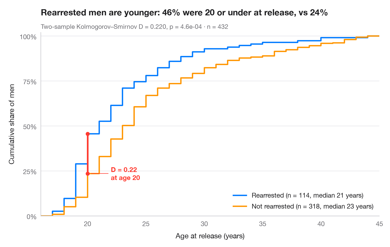
経験累積分布関数(ECDF)は、x軸上の各値について、その値以下の観測値の割合をプロットしたものです。ヒストグラムと違って階級の設定が不要で、あらゆる分位点を直接読み取れます。2つの ECDF を重ねて描くと、両者の垂直方向の最大距離がそのまま2標本 コルモゴロフ・スミルノフ 統計量 D となり、ここでは赤い線分で示しています。
データは、1970年代にメリーランド州の州刑務所から釈放され、1年間追跡された432人の男性(ロッシ、バーク、レニハンの実験)で、lifelines に同梱されています(lifelines.datasets.load_rossi())。1年以内に再逮捕された男性とそうでない男性について、釈放時の年齢を比較しています。scipy.stats.ecdf で曲線を作成し、scipy.stats.ks_2samp で D、その位置、p値を求めています。
コードおよび図中のテキストは英語です。
import matplotlib.pyplot as plt
import numpy as np
from lifelines.datasets import load_rossi
from scipy import stats

# Data: age at release of former prisoners, split by rearrest within one year
df = load_rossi()
groups = {"Rearrested": df.loc[df.arrest == 1, "age"].to_numpy(),
          "Not rearrested": df.loc[df.arrest == 0, "age"].to_numpy()}
palette = ["#007AFF", "#FF9500"]

# Two-sample Kolmogorov–Smirnov test: D is the largest vertical gap
ks = stats.ks_2samp(*groups.values())
x_gap = ks.statistic_location
F = [stats.ecdf(d).cdf for d in groups.values()]
y_gap = [f.evaluate(x_gap) for f in F]

lo, hi = df.age.min() - 1, df.age.max() + 1  # common x-range for both curves
fig, ax = plt.subplots(figsize=(8, 5))
for (name, d), f, c in zip(groups.items(), F, palette):
    ax.step(np.r_[lo, f.quantiles, hi], np.r_[0, f.probabilities, 1], where="post",
            color=c, lw=2, label=f"{name} (n = {len(d)}, median {np.median(d):.0f} years)")

# Mark the KS distance
ax.plot([x_gap, x_gap], y_gap, color="#FF3B30", lw=2.5, solid_capstyle="round", zorder=5)
ax.scatter([x_gap, x_gap], y_gap, color="#FF3B30", s=30, zorder=6)
ax.annotate(f"D = {ks.statistic:.2f}\nat age {x_gap:.0f}", (x_gap + 0.2, min(y_gap)),
            xytext=(x_gap + 2, min(y_gap)), ha="left", va="center", fontsize=10,
            fontweight="semibold", color="#FF3B30",
            arrowprops=dict(arrowstyle="-", color="#FF3B30", lw=0.8, shrinkB=2))

ax.set_xlim(lo, hi)
ax.set_ylim(0, 1.02)
ax.set_yticks(np.linspace(0, 1, 5), [f"{v:.0%}" for v in np.linspace(0, 1, 5)])
ax.set_xlabel("Age at release (years)")
ax.set_ylabel("Cumulative share of men")
ax.legend(loc="lower right")
ax.set_title(f"Rearrested men are younger: {y_gap[0]:.0%} were {x_gap:.0f} or under "
             f"at release, vs {y_gap[1]:.0%}", pad=26)
ax.text(0, 1.02, f"Two-sample Kolmogorov–Smirnov D = {ks.statistic:.3f}, p = {ks.pvalue:.1e}"
        f" · n = {len(df)}", transform=ax.transAxes, fontsize=9.5, color="#6E6E73")
plt.show()
図にはオプションの PyStatlas スタイル を使用しています。同じ見た目にするには plt.style.use("pystatlas.mplstyle") を追加してください。
データの出典
- Rossi recidivism experiment (432 released prisoners). Rossi, P. H., Berk, R. A., & Lenihan, K. J. (1980). Money, Work, and Crime: Some Experimental Results. Academic Press. https://lifelines.readthedocs.io/en/latest/lifelines.datasets.html
Men released from Maryland state prisons in the 1970s, half randomly assigned to financial aid. Distributed with lifelines (lifelines.datasets.load_rossi).
これらの例は統計手法を説明するためのものです。図のタイトルは、この特定のデータ(多くは小規模で、古く、部分的な標本)で図が示す内容を述べたものであり、実質的な問いに対する著者の立場ではありません。解釈、背景、データの質については、ここに挙げた元の出典を参照してください。
引用方法
PyStatlas は Thierry Warin が作成・運営しています。研究や業務に役立った場合は、ぜひ引用してください。
Warin, T. (2026). ECDF comparison. In PyStatlas: A Python Gallery of Statistical Graphics for the Social Sciences. https://warint.github.io/pystatlas/distributions/ecdf-comparison/
@misc{warin2026statlas,
  author       = {Warin, Thierry},
  title        = {PyStatlas: A Python Gallery of Statistical Graphics for the Social Sciences},
  year         = {2026},
  howpublished = {\url{https://warint.github.io/pystatlas/}},
  note         = {Source code: https://github.com/warint/pystatlas}
}