密度曲線付きヒストグラム
ヒストグラム、カーネル密度、当てはめた正規曲線を、分布の形状を表す統計量とともに示します。
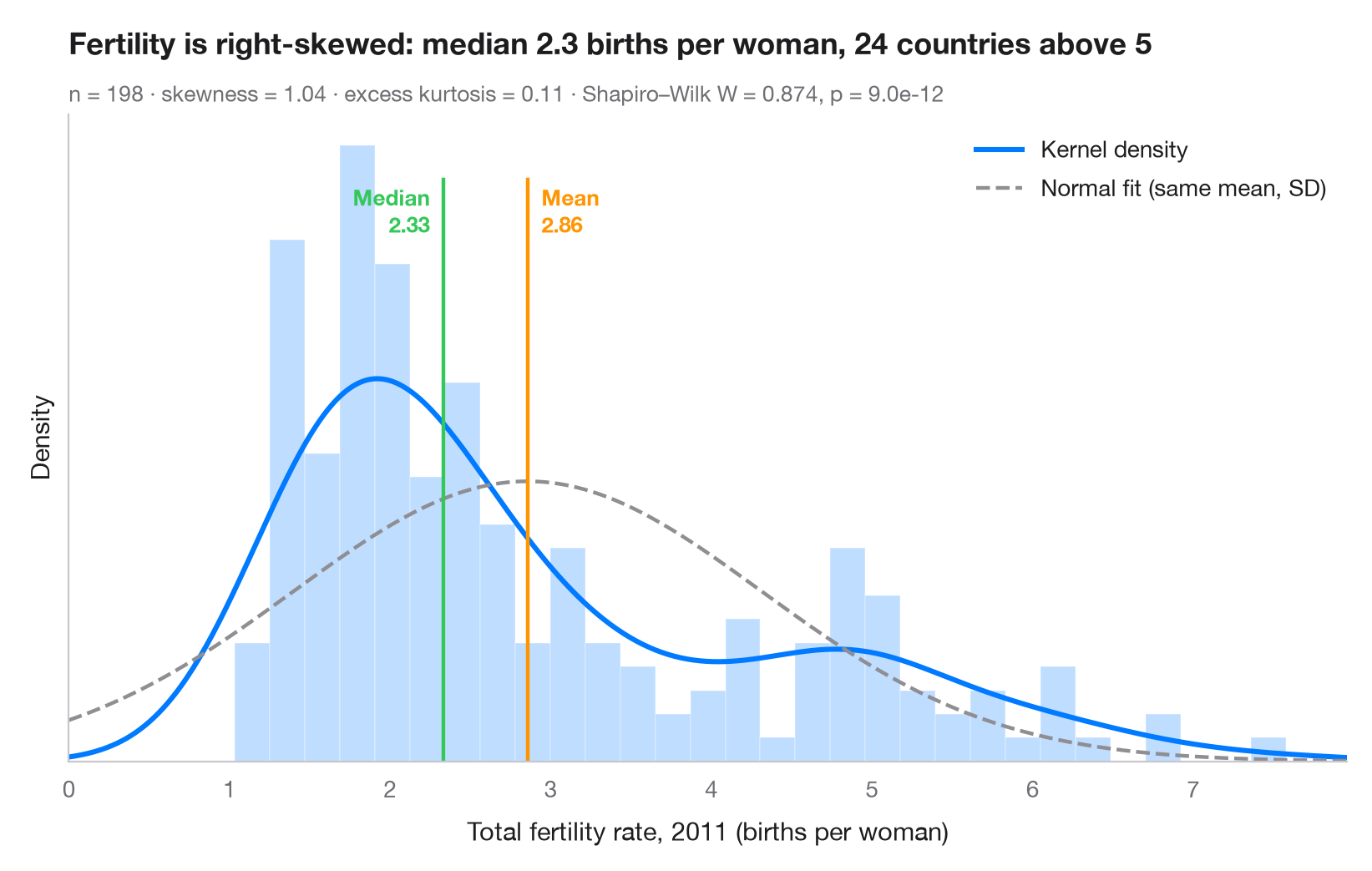
連続変数を調べるときに最初に見るべきグラフです。棒は密度スケールで経験分布を表し、実線はカーネル密度推定(KDE)、破線は同じ平均と標準偏差をもつ正規分布です。2本の曲線が食い違う場合、データは正規分布に従っていません。ここでは出生率の高い国々が作る右に長く伸びた裾が 平均 を 中央値 より大きく引き上げています。
データは世界銀行の合計特殊出生率(女性1人あたりの出生数)で、sm.datasets.fertility(statsmodels)で利用できる最新年である2011年の198の国・地域の値です。5つの地域集計値は除いています。scipy.stats.gaussian_kde で密度を描き、scipy.stats.skew / kurtosis で形状を記述し、scipy.stats.shapiro で正規性を検定しています。
コードおよび図中のテキストは英語です。
import matplotlib.pyplot as plt
import numpy as np
import statsmodels.api as sm
from scipy import stats

# Data: total fertility rate (births per woman) of each country in 2011
wb = sm.datasets.fertility.load_pandas().data
wb = wb[~wb["Country Name"].str.contains("classification|income levels|members|small states")]  # 5 aggregates
x = wb["2011"].dropna().to_numpy()
mean, median, sd = x.mean(), np.median(x), x.std(ddof=1)

# Shape statistics and normality test
skew, kurt = stats.skew(x), stats.kurtosis(x)  # kurtosis: excess, 0 for a normal
W, p = stats.shapiro(x)

fig, ax = plt.subplots(figsize=(8, 5))
ax.hist(x, bins=30, density=True, color="#007AFF", alpha=0.25, edgecolor="white")

# Kernel density estimate and the normal curve with the same mean / SD
grid = np.linspace(0, x.max() * 1.05, 400)
ax.plot(grid, stats.gaussian_kde(x)(grid), color="#007AFF", lw=2.2, label="Kernel density")
ax.plot(grid, stats.norm.pdf(grid, mean, sd), color="#8E8E93", lw=1.6, ls="--",
        label="Normal fit (same mean, SD)")

# Mean and median markers
ymax = ax.get_ylim()[1]
for value, name, color, ha, dx in [(mean, "Mean", "#FF9500", "left", 6),
                                   (median, "Median", "#34C759", "right", -6)]:
    ax.axvline(value, color=color, lw=1.6, ymax=0.9)
    ax.annotate(f"{name}\n{value:.2f}", (value, ymax * 0.9), xytext=(dx, -2),
                textcoords="offset points", ha=ha, va="top", fontsize=9.5,
                fontweight="semibold", color=color)

ax.set_xlim(0, grid[-1])
ax.set_yticks([])
ax.set_ylabel("Density")
ax.set_xlabel("Total fertility rate, 2011 (births per woman)")
ax.legend(loc="upper right")
ax.set_title(f"Fertility is right-skewed: median {median:.1f} births per woman, "
             f"{(x > 5).sum()} countries above 5", pad=26)
ax.text(0, 1.02, f"n = {len(x)} · skewness = {skew:.2f} · excess kurtosis = {kurt:.2f} · "
        f"Shapiro–Wilk W = {W:.3f}, p = {p:.1e}", transform=ax.transAxes,
        fontsize=9.5, color="#6E6E73")
plt.show()
図にはオプションの PyStatlas スタイル を使用しています。同じ見た目にするには plt.style.use("pystatlas.mplstyle") を追加してください。
データの出典
- World Bank fertility rates by country, 1960–2013. World Bank. Fertility rate, total (births per woman), indicator SP.DYN.TFRT.IN. World Development Indicators. https://data.worldbank.org/indicator/SP.DYN.TFRT.IN
Primary sources: UN Population Division, UN Statistical Division, national statistical offices, Eurostat and others. Distributed with statsmodels (sm.datasets.fertility) under the World Bank terms of use.
これらの例は統計手法を説明するためのものです。図のタイトルは、この特定のデータ(多くは小規模で、古く、部分的な標本)で図が示す内容を述べたものであり、実質的な問いに対する著者の立場ではありません。解釈、背景、データの質については、ここに挙げた元の出典を参照してください。
引用方法
PyStatlas は Thierry Warin が作成・運営しています。研究や業務に役立った場合は、ぜひ引用してください。
Warin, T. (2026). Histogram with density. In PyStatlas: A Python Gallery of Statistical Graphics for the Social Sciences. https://warint.github.io/pystatlas/distributions/histogram-density/
@misc{warin2026statlas,
  author       = {Warin, Thierry},
  title        = {PyStatlas: A Python Gallery of Statistical Graphics for the Social Sciences},
  year         = {2026},
  howpublished = {\url{https://warint.github.io/pystatlas/}},
  note         = {Source code: https://github.com/warint/pystatlas}
}