Histogram with density
Histogram, kernel density and fitted normal curve, with shape statistics.
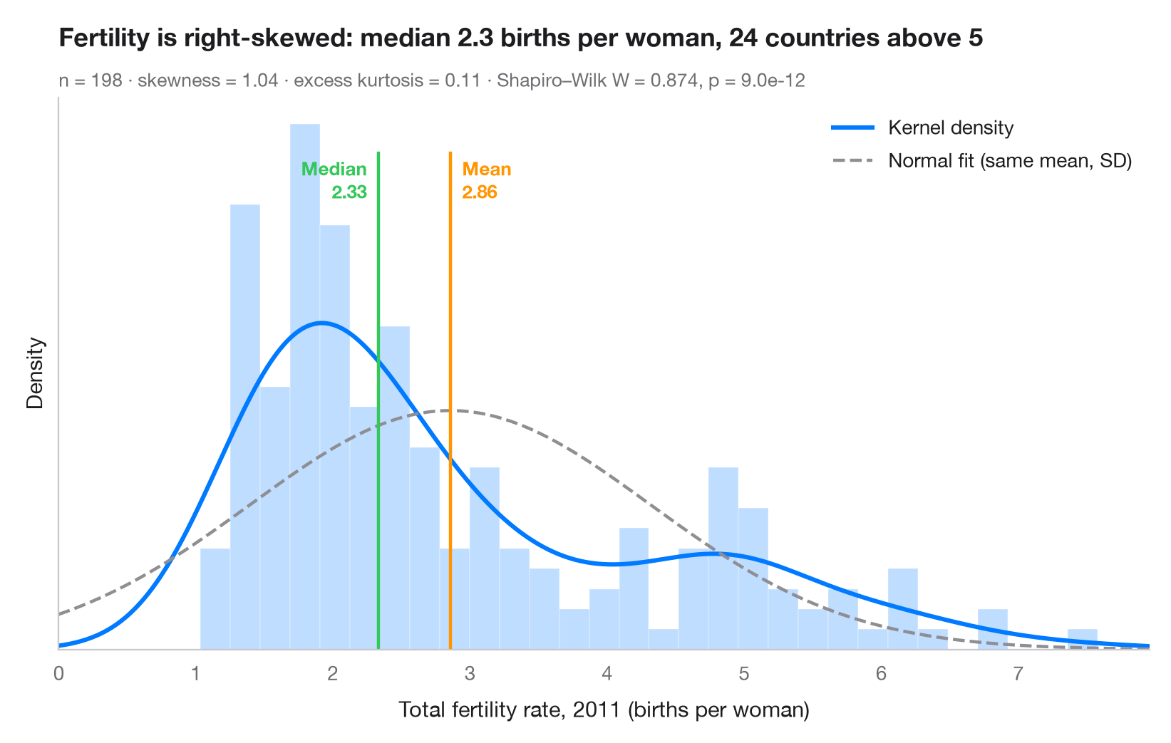
The first look at any continuous variable. Bars show the empirical distribution on a density scale, the solid curve is a kernel density estimate (KDE) and the dashed curve is the normal distribution with the same mean and standard deviation. When the two curves disagree, the data are not normal — here the long right tail of high-fertility countries pulls the mean above the median.
Data are the World Bank total fertility rate (births per woman) of 198
countries and territories in 2011, the latest year available in
sm.datasets.fertility (statsmodels); the five regional aggregates are
dropped. scipy.stats.gaussian_kde draws the density,
scipy.stats.skew / kurtosis describe the shape and scipy.stats.shapiro
tests normality.
import matplotlib.pyplot as plt
import numpy as np
import statsmodels.api as sm
from scipy import stats

# Data: total fertility rate (births per woman) of each country in 2011
wb = sm.datasets.fertility.load_pandas().data
wb = wb[~wb["Country Name"].str.contains("classification|income levels|members|small states")]  # 5 aggregates
x = wb["2011"].dropna().to_numpy()
mean, median, sd = x.mean(), np.median(x), x.std(ddof=1)

# Shape statistics and normality test
skew, kurt = stats.skew(x), stats.kurtosis(x)  # kurtosis: excess, 0 for a normal
W, p = stats.shapiro(x)

fig, ax = plt.subplots(figsize=(8, 5))
ax.hist(x, bins=30, density=True, color="#007AFF", alpha=0.25, edgecolor="white")

# Kernel density estimate and the normal curve with the same mean / SD
grid = np.linspace(0, x.max() * 1.05, 400)
ax.plot(grid, stats.gaussian_kde(x)(grid), color="#007AFF", lw=2.2, label="Kernel density")
ax.plot(grid, stats.norm.pdf(grid, mean, sd), color="#8E8E93", lw=1.6, ls="--",
        label="Normal fit (same mean, SD)")

# Mean and median markers
ymax = ax.get_ylim()[1]
for value, name, color, ha, dx in [(mean, "Mean", "#FF9500", "left", 6),
                                   (median, "Median", "#34C759", "right", -6)]:
    ax.axvline(value, color=color, lw=1.6, ymax=0.9)
    ax.annotate(f"{name}\n{value:.2f}", (value, ymax * 0.9), xytext=(dx, -2),
                textcoords="offset points", ha=ha, va="top", fontsize=9.5,
                fontweight="semibold", color=color)

ax.set_xlim(0, grid[-1])
ax.set_yticks([])
ax.set_ylabel("Density")
ax.set_xlabel("Total fertility rate, 2011 (births per woman)")
ax.legend(loc="upper right")
ax.set_title(f"Fertility is right-skewed: median {median:.1f} births per woman, "
             f"{(x > 5).sum()} countries above 5", pad=26)
ax.text(0, 1.02, f"n = {len(x)} · skewness = {skew:.2f} · excess kurtosis = {kurt:.2f} · "
        f"Shapiro–Wilk W = {W:.3f}, p = {p:.1e}", transform=ax.transAxes,
        fontsize=9.5, color="#6E6E73")
plt.show()
Figures use the optional PyStatlas style: add plt.style.use("pystatlas.mplstyle") to match the look exactly.
Data source
- World Bank fertility rates by country, 1960–2013. World Bank. Fertility rate, total (births per woman), indicator SP.DYN.TFRT.IN. World Development Indicators. https://data.worldbank.org/indicator/SP.DYN.TFRT.IN
Primary sources: UN Population Division, UN Statistical Division, national statistical offices, Eurostat and others. Distributed with statsmodels (sm.datasets.fertility) under the World Bank terms of use.
The examples illustrate statistical methods. Their titles describe what each figure shows in these particular data — often a small, dated or partial sample — not the author's position on the substantive question. For interpretation, context and data quality, rely on the original sources cited here.
How to cite
PyStatlas is created and maintained by Thierry Warin. If it helped your work, please cite it.
Warin, T. (2026). Histogram with density. In PyStatlas: A Python Gallery of Statistical Graphics for the Social Sciences. https://warint.github.io/pystatlas/distributions/histogram-density/
@misc{warin2026statlas,
  author       = {Warin, Thierry},
  title        = {PyStatlas: A Python Gallery of Statistical Graphics for the Social Sciences},
  year         = {2026},
  howpublished = {\url{https://warint.github.io/pystatlas/}},
  note         = {Source code: https://github.com/warint/pystatlas}
}More in Distributions
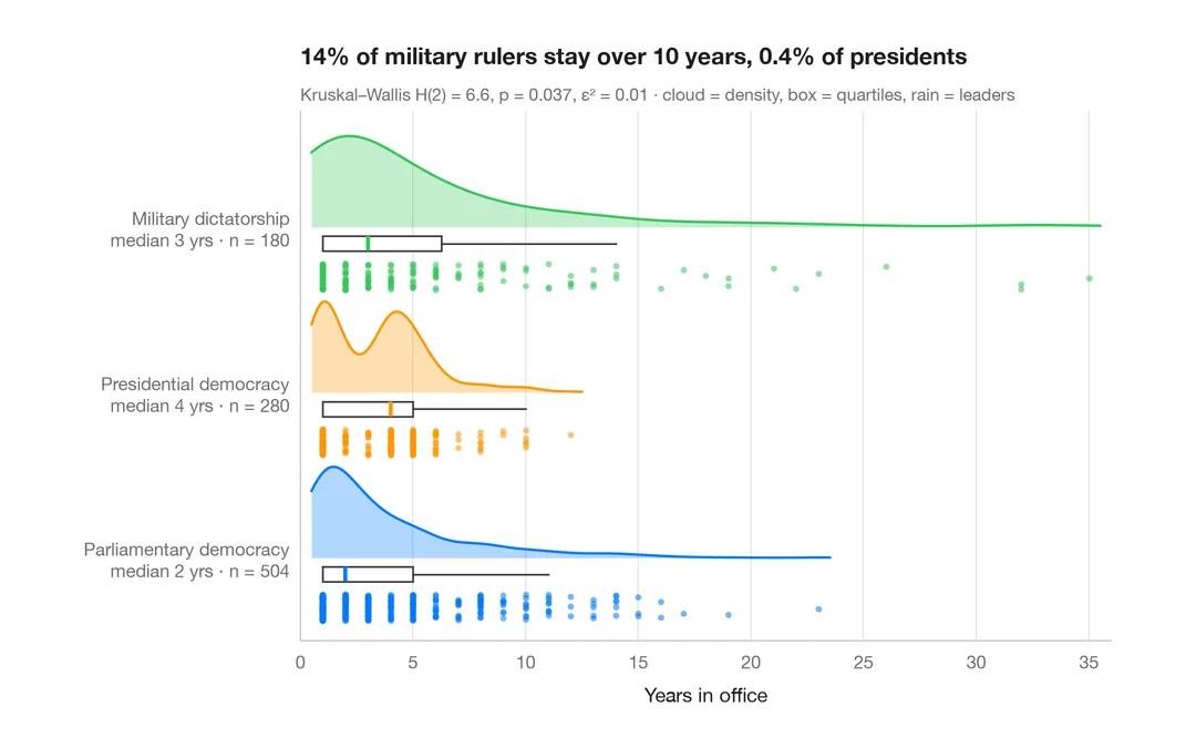
Raincloud plot
Half violin, box plot and raw points per group, drawn horizontally.
ggdist::stat_halfeye() / ggrain::geom_rain()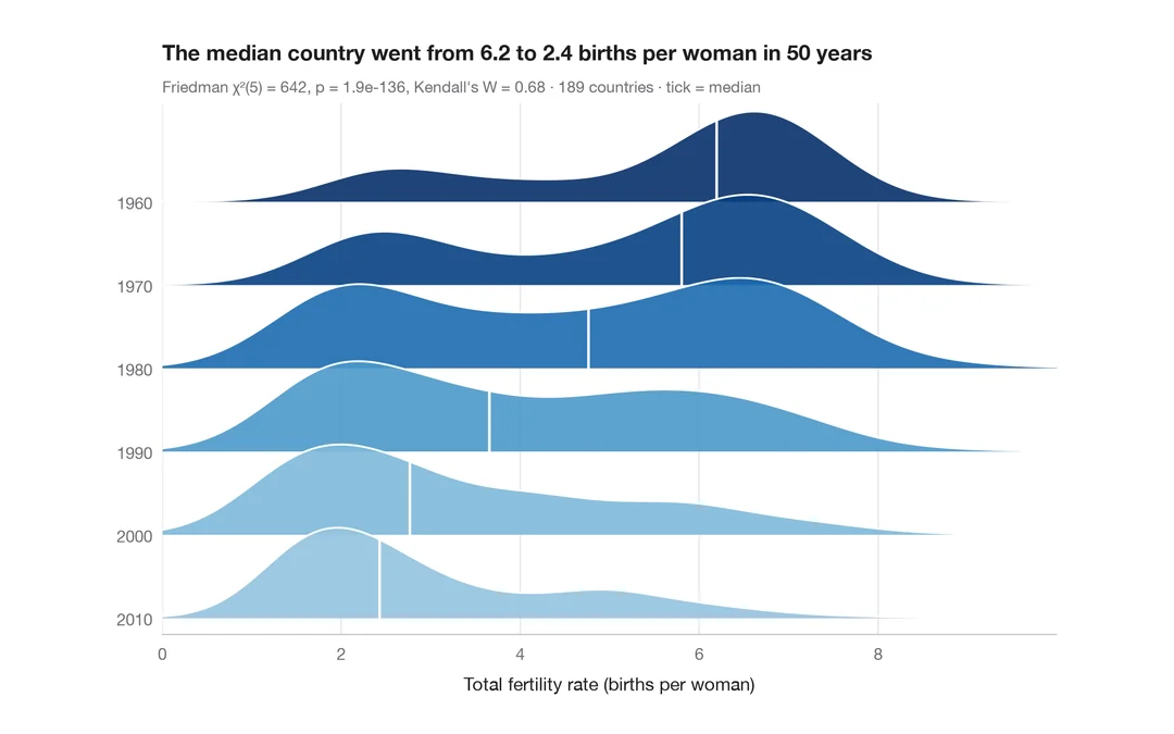
Ridgeline plot
Overlapping density curves to compare one distribution across many groups.
ggridges::geom_density_ridges()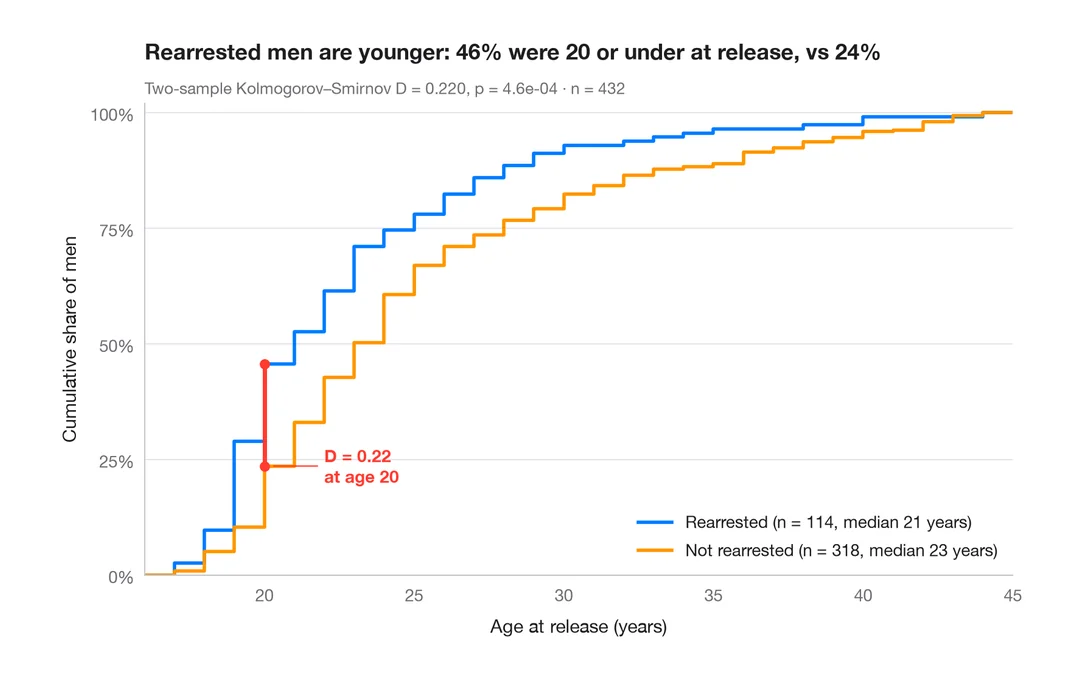
ECDF comparison
Empirical cumulative distributions of two groups, with the Kolmogorov–Smirnov gap.
ggplot2::stat_ecdf()