ECDF comparison

Warin, Thierry

Empirical cumulative distributions of two groups, with the Kolmogorov–Smirnov gap.

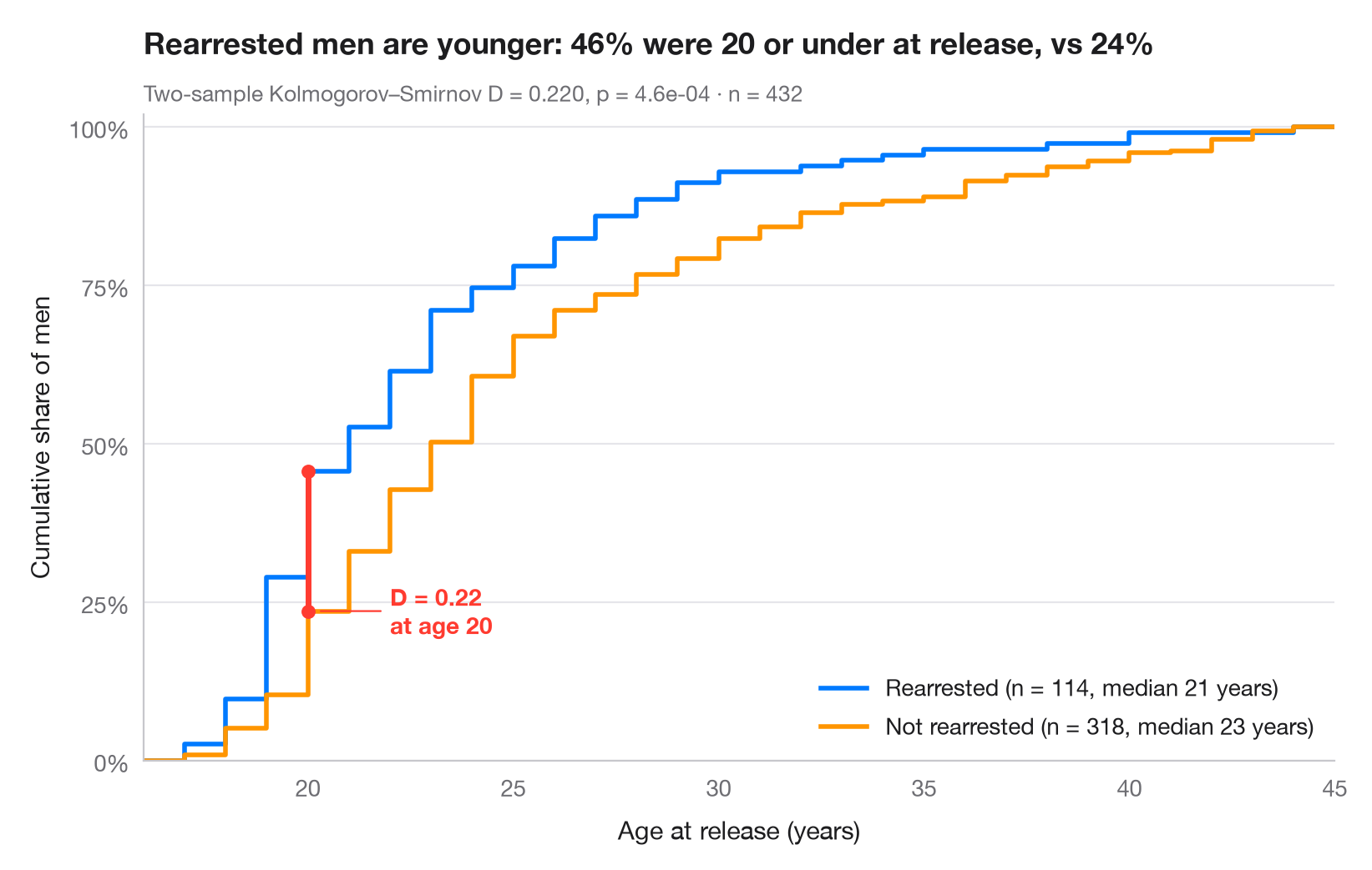
An empirical cumulative distribution function (ECDF) plots, for every value on the x-axis, the share of observations at or below it. Unlike a histogram it needs no bins, and every quantile can be read off directly. When two ECDFs are drawn together, the largest vertical distance between them is exactly the two-sample Kolmogorov–Smirnov statistic D, drawn here as a red segment.

Data are the 432 men released from Maryland state prisons in the 1970s and followed for one year (Rossi, Berk & Lenihan's experiment), bundled with lifelines (lifelines.datasets.load_rossi()): age at release, for men rearrested within the year versus those who were not. scipy.stats.ecdf builds the curves and scipy.stats.ks_2samp returns D, its location and the p-value.

ecdf-comparison.py · 42 lines

Download GitHub

import matplotlib.pyplot as plt
import numpy as np
from lifelines.datasets import load_rossi
from scipy import stats

# Data: age at release of former prisoners, split by rearrest within one year
df = load_rossi()
groups = {"Rearrested": df.loc[df.arrest == 1, "age"].to_numpy(),
          "Not rearrested": df.loc[df.arrest == 0, "age"].to_numpy()}
palette = ["#007AFF", "#FF9500"]

# Two-sample Kolmogorov–Smirnov test: D is the largest vertical gap
ks = stats.ks_2samp(*groups.values())
x_gap = ks.statistic_location
F = [stats.ecdf(d).cdf for d in groups.values()]
y_gap = [f.evaluate(x_gap) for f in F]

lo, hi = df.age.min() - 1, df.age.max() + 1  # common x-range for both curves
fig, ax = plt.subplots(figsize=(8, 5))
for (name, d), f, c in zip(groups.items(), F, palette):
    ax.step(np.r_[lo, f.quantiles, hi], np.r_[0, f.probabilities, 1], where="post",
            color=c, lw=2, label=f"{name} (n = {len(d)}, median {np.median(d):.0f} years)")

# Mark the KS distance
ax.plot([x_gap, x_gap], y_gap, color="#FF3B30", lw=2.5, solid_capstyle="round", zorder=5)
ax.scatter([x_gap, x_gap], y_gap, color="#FF3B30", s=30, zorder=6)
ax.annotate(f"D = {ks.statistic:.2f}\nat age {x_gap:.0f}", (x_gap + 0.2, min(y_gap)),
            xytext=(x_gap + 2, min(y_gap)), ha="left", va="center", fontsize=10,
            fontweight="semibold", color="#FF3B30",
            arrowprops=dict(arrowstyle="-", color="#FF3B30", lw=0.8, shrinkB=2))

ax.set_xlim(lo, hi)
ax.set_ylim(0, 1.02)
ax.set_yticks(np.linspace(0, 1, 5), [f"{v:.0%}" for v in np.linspace(0, 1, 5)])
ax.set_xlabel("Age at release (years)")
ax.set_ylabel("Cumulative share of men")
ax.legend(loc="lower right")
ax.set_title(f"Rearrested men are younger: {y_gap[0]:.0%} were {x_gap:.0f} or under "
             f"at release, vs {y_gap[1]:.0%}", pad=26)
ax.text(0, 1.02, f"Two-sample Kolmogorov–Smirnov D = {ks.statistic:.3f}, p = {ks.pvalue:.1e}"
        f" · n = {len(df)}", transform=ax.transAxes, fontsize=9.5, color="#6E6E73")
plt.show()

Figures use the optional PyStatlas style: add plt.style.use("pystatlas.mplstyle") to match the look exactly.

Data source

Rossi recidivism experiment (432 released prisoners). Rossi, P. H., Berk, R. A., & Lenihan, K. J. (1980). Money, Work, and Crime: Some Experimental Results. Academic Press. https://lifelines.readthedocs.io/en/latest/lifelines.datasets.html
Men released from Maryland state prisons in the 1970s, half randomly assigned to financial aid. Distributed with lifelines (lifelines.datasets.load_rossi).

The examples illustrate statistical methods. Their titles describe what each figure shows in these particular data — often a small, dated or partial sample — not the author's position on the substantive question. For interpretation, context and data quality, rely on the original sources cited here.

How to cite

PyStatlas is created and maintained by Thierry Warin. If it helped your work, please cite it.

Warin, T. (2026). ECDF comparison. In PyStatlas: A Python Gallery of Statistical Graphics for the Social Sciences. https://warint.github.io/pystatlas/distributions/ecdf-comparison/

@misc{warin2026statlas,
  author       = {Warin, Thierry},
  title        = {PyStatlas: A Python Gallery of Statistical Graphics for the Social Sciences},
  year         = {2026},
  howpublished = {\url{https://warint.github.io/pystatlas/}},
  note         = {Source code: https://github.com/warint/pystatlas}
}

More in Distributions

Distributions

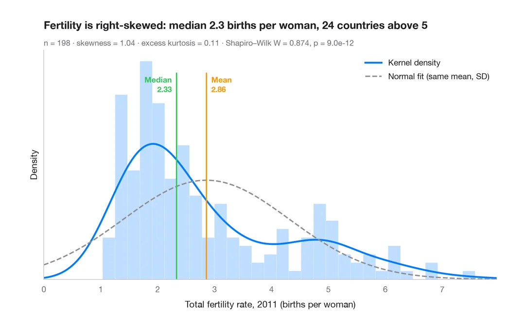
Histogram with density

Histogram, kernel density and fitted normal curve, with shape statistics.

ggplot2::geom_histogram() + geom_density()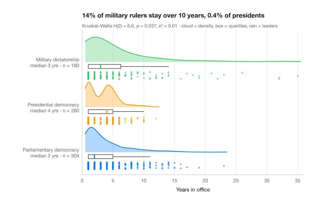

Distributions

Raincloud plot

Half violin, box plot and raw points per group, drawn horizontally.

ggdist::stat_halfeye() / ggrain::geom_rain()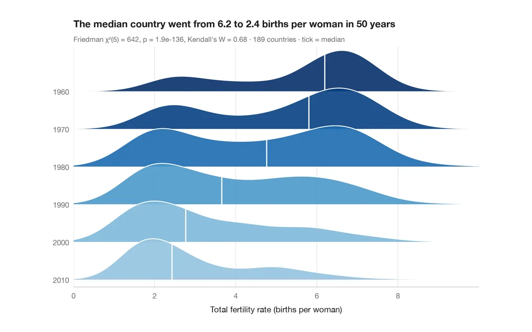

Distributions

Ridgeline plot

Overlapping density curves to compare one distribution across many groups.

ggridges::geom_density_ridges()