Q–Q plot with confidence band — PyStatlas: A Python Gallery of Statistical Graphics for the Social Sciences

Warin, Thierry

信頼帯付き Q–Q プロット

元の変数と対数変換した変数について、95% 包絡線付きの正規 Q–Q プロットを描きます。

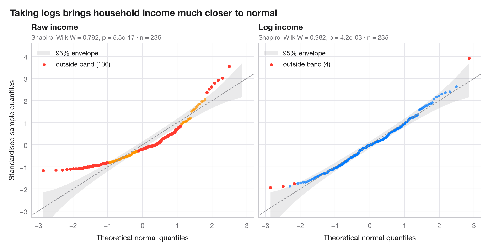
Q–Q プロット（分位点–分位点プロット）は、並べ替えて標準化したデータを、正規分布から得られる分位点に対してプロットしたものです。正規分布に従うデータは対角線上に並び、弓なりに曲がったパターンは歪みを意味します。網掛けの帯は、正規順序統計量のベータ分布から構成した各点ごとの 95% 包絡線で、その外側にある点は偶然では説明しにくいほど極端な値です。

データはベルギーの労働者世帯 235 世帯の世帯収入です（エンゲルの食費データ、statsmodels に同梱）。左のパネルは元の収入、右のパネルはその対数を示しています。分位点は scipy.stats.norm.ppf、包絡線は scipy.stats.beta.ppf で求め、各パネルにシャピロ・ウィルク検定の結果を示しています。

コードおよび図中のテキストは英語です。

qq-plot.py · 43 行

ダウンロード GitHub

import matplotlib.pyplot as plt
import numpy as np
import statsmodels.api as sm
from scipy import stats

# Data: household income, raw and log-transformed
income = sm.datasets.engel.load_pandas().data["income"].to_numpy()
samples = {"Raw income": income, "Log income": np.log(income)}
palette = ["#FF9500", "#007AFF"]

fig, axes = plt.subplots(1, 2, figsize=(10, 5), sharex=True, sharey=True)
for ax, (name, x), c in zip(axes, samples.items(), palette):
    n = len(x)
    z = np.sort((x - x.mean()) / x.std(ddof=1))      # standardised sample quantiles
    pp = (np.arange(1, n + 1) - 0.5) / n              # plotting positions
    theo = stats.norm.ppf(pp)                         # theoretical normal quantiles

    # 95% pointwise envelope: order statistic i of a uniform sample is Beta(i, n-i+1)
    i = np.arange(1, n + 1)
    lo = stats.norm.ppf(stats.beta.ppf(0.025, i, n - i + 1))
    hi = stats.norm.ppf(stats.beta.ppf(0.975, i, n - i + 1))
    outside = (z < lo) | (z > hi)

    ax.fill_between(theo, lo, hi, color="#8E8E93", alpha=0.18, lw=0, label="95% envelope")
    ax.plot([-3.5, 3.5], [-3.5, 3.5], color="#8E8E93", lw=1, ls="--")
    ax.scatter(theo[~outside], z[~outside], s=16, color=c, alpha=0.7, lw=0)
    ax.scatter(theo[outside], z[outside], s=22, color="#FF3B30", lw=0,
               label=f"outside band ({outside.sum()})")

    W, p = stats.shapiro(x)
    ax.set_title(name, pad=20, fontsize=12)
    ax.text(0, 1.02, f"Shapiro–Wilk W = {W:.3f}, p = {p:.1e} · n = {n}",
            transform=ax.transAxes, fontsize=9.5, color="#6E6E73")
    ax.legend(loc="upper left")
    ax.grid(axis="x")
    ax.set_xlabel("Theoretical normal quantiles")

axes[0].set_ylabel("Standardised sample quantiles")
axes[0].set_xlim(-3.2, 3.2)
axes[0].set_ylim(-3.3, 4.6)
fig.suptitle("Taking logs brings household income much closer to normal",
             x=0.01, ha="left", fontsize=14)
plt.show()

図にはオプションの PyStatlas スタイルを使用しています。同じ見た目にするには plt.style.use("pystatlas.mplstyle") を追加してください。

データの出典

Engel's Belgian household budgets (235 families). Koenker, R., & Bassett, G. (1982). Robust tests for heteroscedasticity based on regression quantiles. Econometrica, 50(1), 43–61. https://doi.org/10.2307/1912528
Engel's (1857) household budget data as used by Koenker and Bassett and distributed with R's quantreg; in statsmodels as sm.datasets.engel; public domain.

これらの例は統計手法を説明するためのものです。図のタイトルは、この特定のデータ（多くは小規模で、古く、部分的な標本）で図が示す内容を述べたものであり、実質的な問いに対する著者の立場ではありません。解釈、背景、データの質については、ここに挙げた元の出典を参照してください。

引用方法

PyStatlas は Thierry Warin が作成・運営しています。研究や業務に役立った場合は、ぜひ引用してください。

Warin, T. (2026). Q–Q plot with confidence band. In PyStatlas: A Python Gallery of Statistical Graphics for the Social Sciences. https://warint.github.io/pystatlas/distributions/qq-plot/

@misc{warin2026statlas,
  author       = {Warin, Thierry},
  title        = {PyStatlas: A Python Gallery of Statistical Graphics for the Social Sciences},
  year         = {2026},
  howpublished = {\url{https://warint.github.io/pystatlas/}},
  note         = {Source code: https://github.com/warint/pystatlas}
}