带置信带的 Q–Q 图
带 95% 包络带的正态 Q–Q 图,分别展示原始变量与对数变换后的变量。
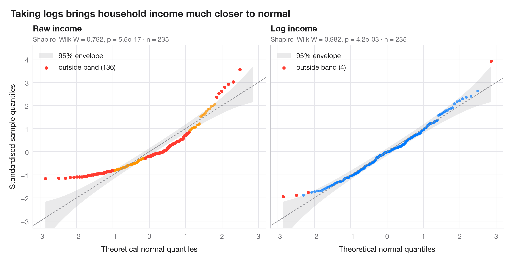
分位数–分位数图将排序并标准化后的数据与正态分布对应的理论分位数相对照。正态数据落在对角线上;弯曲的香蕉形模式则意味着偏态。阴影带是基于正态次序统计量的 Beta 分布构建的 95% 逐点包络,落在其外的点比随机波动所能解释的更为极端。
数据为 235 个比利时工人家庭的收入(Engel 食品支出数据,statsmodels 自带)。左图为原始收入,右图为其对数。分位数由 scipy.stats.norm.ppf 计算,包络由 scipy.stats.beta.ppf 计算,每个子图均报告 Shapiro–Wilk 检验。
代码及图中文字均为英文。
import matplotlib.pyplot as plt
import numpy as np
import statsmodels.api as sm
from scipy import stats

# Data: household income, raw and log-transformed
income = sm.datasets.engel.load_pandas().data["income"].to_numpy()
samples = {"Raw income": income, "Log income": np.log(income)}
palette = ["#FF9500", "#007AFF"]

fig, axes = plt.subplots(1, 2, figsize=(10, 5), sharex=True, sharey=True)
for ax, (name, x), c in zip(axes, samples.items(), palette):
    n = len(x)
    z = np.sort((x - x.mean()) / x.std(ddof=1))      # standardised sample quantiles
    pp = (np.arange(1, n + 1) - 0.5) / n              # plotting positions
    theo = stats.norm.ppf(pp)                         # theoretical normal quantiles

    # 95% pointwise envelope: order statistic i of a uniform sample is Beta(i, n-i+1)
    i = np.arange(1, n + 1)
    lo = stats.norm.ppf(stats.beta.ppf(0.025, i, n - i + 1))
    hi = stats.norm.ppf(stats.beta.ppf(0.975, i, n - i + 1))
    outside = (z < lo) | (z > hi)

    ax.fill_between(theo, lo, hi, color="#8E8E93", alpha=0.18, lw=0, label="95% envelope")
    ax.plot([-3.5, 3.5], [-3.5, 3.5], color="#8E8E93", lw=1, ls="--")
    ax.scatter(theo[~outside], z[~outside], s=16, color=c, alpha=0.7, lw=0)
    ax.scatter(theo[outside], z[outside], s=22, color="#FF3B30", lw=0,
               label=f"outside band ({outside.sum()})")

    W, p = stats.shapiro(x)
    ax.set_title(name, pad=20, fontsize=12)
    ax.text(0, 1.02, f"Shapiro–Wilk W = {W:.3f}, p = {p:.1e} · n = {n}",
            transform=ax.transAxes, fontsize=9.5, color="#6E6E73")
    ax.legend(loc="upper left")
    ax.grid(axis="x")
    ax.set_xlabel("Theoretical normal quantiles")

axes[0].set_ylabel("Standardised sample quantiles")
axes[0].set_xlim(-3.2, 3.2)
axes[0].set_ylim(-3.3, 4.6)
fig.suptitle("Taking logs brings household income much closer to normal",
             x=0.01, ha="left", fontsize=14)
plt.show()
图表使用了可选的 PyStatlas 样式:添加 plt.style.use("pystatlas.mplstyle") 即可完全还原其外观。
数据来源
- Engel's Belgian household budgets (235 families). Koenker, R., & Bassett, G. (1982). Robust tests for heteroscedasticity based on regression quantiles. Econometrica, 50(1), 43–61. https://doi.org/10.2307/1912528
Engel's (1857) household budget data as used by Koenker and Bassett and distributed with R's quantreg; in statsmodels as sm.datasets.engel; public domain.
这些示例用于说明统计方法。图表标题描述的是该图在这些特定数据中呈现的内容——这些数据往往样本较小、年代较早或并不完整——而不是作者对实质问题的立场。关于解释、背景和数据质量,请以此处引用的原始来源为准。
如何引用
PyStatlas 由 Thierry Warin 创建并维护。如果它对你的工作有所帮助,敬请引用。
Warin, T. (2026). Q–Q plot with confidence band. In PyStatlas: A Python Gallery of Statistical Graphics for the Social Sciences. https://warint.github.io/pystatlas/distributions/qq-plot/
@misc{warin2026statlas,
  author       = {Warin, Thierry},
  title        = {PyStatlas: A Python Gallery of Statistical Graphics for the Social Sciences},
  year         = {2026},
  howpublished = {\url{https://warint.github.io/pystatlas/}},
  note         = {Source code: https://github.com/warint/pystatlas}
}