Within-subjects comparison
Repeated measures with one line per subject, means, rm-ANOVA and paired tests.
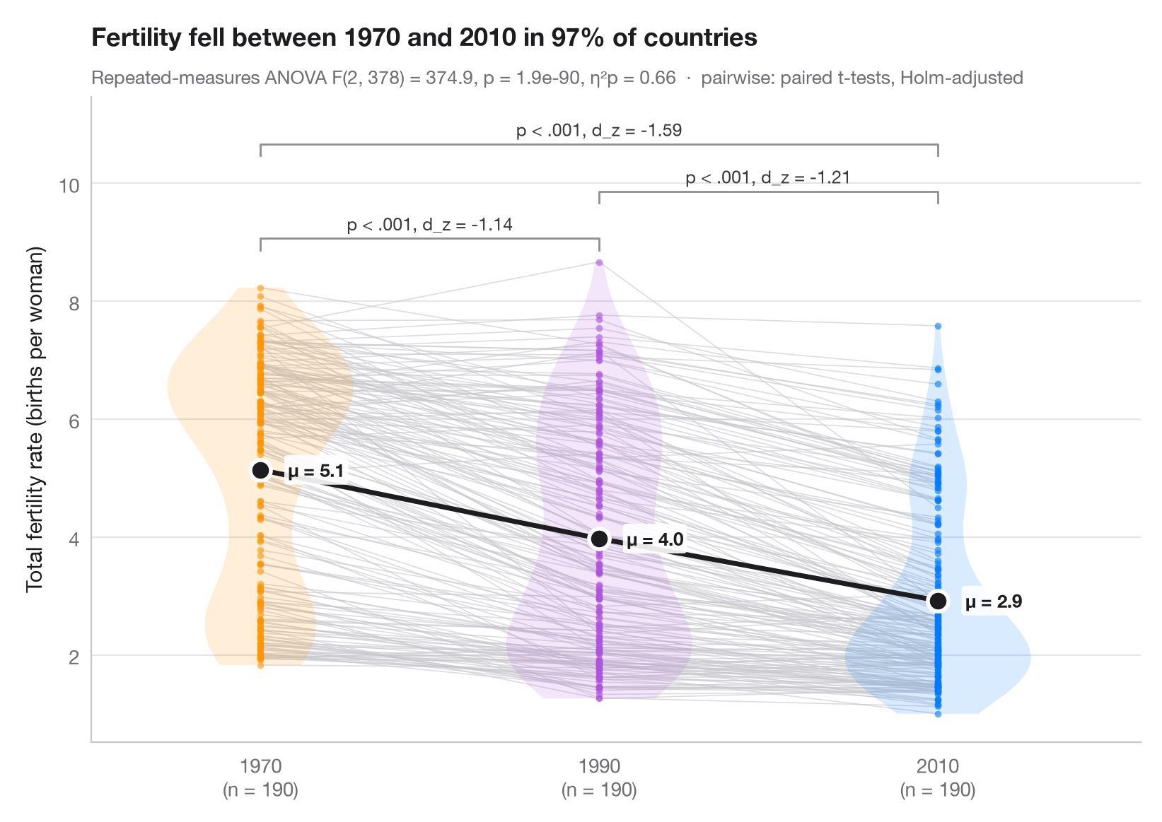
When the same units are measured under every condition, the interesting variation is within each unit. Thin grey lines join each country's measurements, so you can see whether almost every country moves in the same direction; violins show the distribution per year and the large dots (joined by a dark line) are the yearly means.
Data are the World Bank total fertility rate (births per woman) bundled with
statsmodels (sm.datasets.fertility): the 190 countries with a value in
1970, 1990 and 2010 (regional aggregates dropped), so each country is
measured three times. The subtitle reports a one-way repeated-measures ANOVA
(statsmodels.stats.anova.AnovaRM) with partial η², and the brackets show
Holm-corrected paired t-tests (scipy.stats.ttest_rel) with Cohen's d_z
(negative = fertility fell).
from itertools import combinations

import matplotlib.pyplot as plt
import numpy as np
import pandas as pd
import statsmodels.api as sm
from scipy import stats
from statsmodels.stats.anova import AnovaRM
from statsmodels.stats.multitest import multipletests

# Data: fertility of the same countries in 1970, 1990 and 2010 (births per woman)
wb = sm.datasets.fertility.load_pandas().data
wb = wb[~wb["Country Name"].str.contains("classification|income levels|members|small states")]  # 5 aggregates
conditions = ["1970", "1990", "2010"]
wide = wb[conditions].dropna().reset_index(drop=True)
n = len(wide)
long = wide.rename_axis("id").reset_index().melt("id", var_name="condition", value_name="tfr")

# Repeated-measures ANOVA + partial eta squared
aov = AnovaRM(long, "tfr", "id", within=["condition"]).fit().anova_table.iloc[0]
eta_p = aov["F Value"] * aov["Num DF"] / (aov["F Value"] * aov["Num DF"] + aov["Den DF"])

# Pairwise paired t-tests (Holm) with Cohen's d_z
pairs = list(combinations(range(3), 2))
tests = [stats.ttest_rel(wide.iloc[:, j], wide.iloc[:, i]) for i, j in pairs]
adj_p = multipletests([t.pvalue for t in tests], method="holm")[1]
dz = [(wide.iloc[:, j] - wide.iloc[:, i]).mean() / (wide.iloc[:, j] - wide.iloc[:, i]).std()
      for i, j in pairs]

fig, ax = plt.subplots(figsize=(8, 5.6))
palette = ["#FF9500", "#AF52DE", "#007AFF"]
x = np.arange(3)
for _, row in wide.iterrows():                      # one line per subject
    ax.plot(x, row.values, color="#C7C7CC", lw=0.6, alpha=0.6, zorder=1)
for i, c in enumerate(palette):
    v = ax.violinplot(wide.iloc[:, i], positions=[i], widths=0.55, showextrema=False)
    v["bodies"][0].set(facecolor=c, alpha=0.15, edgecolor="none")
    ax.scatter(np.full(n, i), wide.iloc[:, i], s=12, color=c, alpha=0.6, lw=0, zorder=2)
means = wide.mean()
ax.plot(x, means, color="#1D1D1F", lw=2.5, zorder=3)
ax.scatter(x, means, s=110, color="#1D1D1F", edgecolor="white", lw=2, zorder=4)
for i, m in enumerate(means):
    ax.annotate(f"μ = {m:.1f}", (i, m), xytext=(14, 0), textcoords="offset points", va="center",
                fontsize=9.5, fontweight="semibold", color="#1D1D1F",
                bbox=dict(boxstyle="round,pad=0.2", fc="white", ec="none", alpha=0.9), zorder=5)

# Significance brackets
top, step = wide.values.max() + 0.4, 0.8
for h, ((i, j), p, d) in enumerate(sorted(zip(pairs, adj_p, dz), key=lambda t: t[0][1] - t[0][0])):
    y = top + h * step
    ax.plot([i, i, j, j], [y - 0.2, y, y, y - 0.2], color="#8E8E93", lw=1)
    label = "p < .001" if p < 0.001 else f"p = {p:.3f}"
    ax.text((i + j) / 2, y + 0.07, f"{label}, d_z = {d:.2f}", ha="center", va="bottom",
            fontsize=9, color="#3A3A3C")

ax.set_xticks(x, [f"{c}\n(n = {n})" for c in conditions])
ax.set_xlim(-0.5, 2.6)
ax.set_ylim(top=top + 3 * step)
ax.set_ylabel("Total fertility rate (births per woman)")
fell = (wide["2010"] < wide["1970"]).mean()
ax.set_title(f"Fertility fell between 1970 and 2010 in {fell:.0%} of countries", pad=26)
ax.text(0, 1.02, f"Repeated-measures ANOVA F({aov['Num DF']:.0f}, {aov['Den DF']:.0f}) = "
        f"{aov['F Value']:.1f}, p = {aov['Pr > F']:.1e}, η²p = {eta_p:.2f}  ·  "
        "pairwise: paired t-tests, Holm-adjusted", transform=ax.transAxes,
        fontsize=9.5, color="#6E6E73")
plt.show()
Figures use the optional PyStatlas style: add plt.style.use("pystatlas.mplstyle") to match the look exactly.
Data source
- World Bank fertility rates by country, 1960–2013. World Bank. Fertility rate, total (births per woman), indicator SP.DYN.TFRT.IN. World Development Indicators. https://data.worldbank.org/indicator/SP.DYN.TFRT.IN
Primary sources: UN Population Division, UN Statistical Division, national statistical offices, Eurostat and others. Distributed with statsmodels (sm.datasets.fertility) under the World Bank terms of use.
The examples illustrate statistical methods. Their titles describe what each figure shows in these particular data — often a small, dated or partial sample — not the author's position on the substantive question. For interpretation, context and data quality, rely on the original sources cited here.
How to cite
PyStatlas is created and maintained by Thierry Warin. If it helped your work, please cite it.
Warin, T. (2026). Within-subjects comparison. In PyStatlas: A Python Gallery of Statistical Graphics for the Social Sciences. https://warint.github.io/pystatlas/group-comparisons/within-subjects/
@misc{warin2026statlas,
  author       = {Warin, Thierry},
  title        = {PyStatlas: A Python Gallery of Statistical Graphics for the Social Sciences},
  year         = {2026},
  howpublished = {\url{https://warint.github.io/pystatlas/}},
  note         = {Source code: https://github.com/warint/pystatlas}
}More in Group comparisons
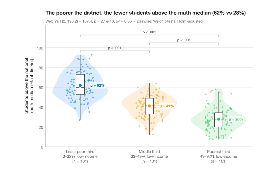
Between-groups comparison
Violin + box + points with Welch's ANOVA, effect size and pairwise tests.
ggstatsplot::ggbetweenstats()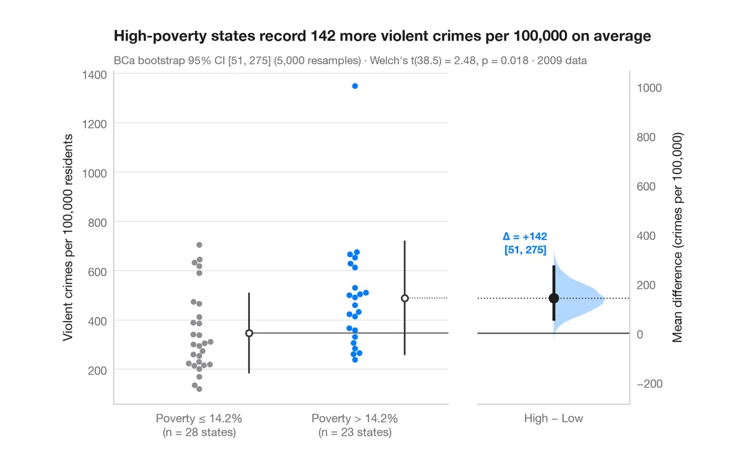
Estimation plot
Raw data of two groups plus the mean difference and its bootstrap 95% CI.
dabestr::dabest() + plot()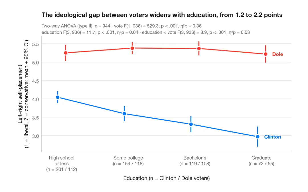
Interaction plot
Group means with 95% confidence intervals for two factors, with a two-way ANOVA.
ggpubr::ggline(add = "mean_ci") / ggstats