Estimation plot
Raw data of two groups plus the mean difference and its bootstrap 95% CI.
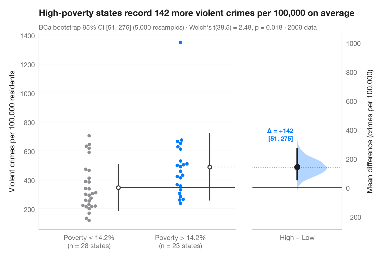
The Gardner–Altman estimation plot puts the effect size, not the p-value, at the centre. The left axis shows every observation of both groups; the right, floating axis is anchored so that its zero sits at the reference-group mean. On it, the bootstrap distribution of the mean difference is drawn as a half violin, with the point estimate and its 95% confidence interval as a dot and a bar.
Data are the 50 US states plus the District of Columbia in 2009, bundled with
statsmodels (sm.datasets.statecrime): the violent-crime rate per
100,000 residents, for the 23 states whose poverty rate is above the median
state (14.2%) versus the 28 at or below it. The comparison is
observational, not an experiment: it measures how large the gap is, not
what causes it. The 95% CI is a bias-corrected and accelerated (BCa)
bootstrap from scipy.stats.bootstrap, and the subtitle adds Welch's
t-test (scipy.stats.ttest_ind); the vertical line beside each swarm is the
group mean ± 1 SD, and the swarm comes from seaborn.swarmplot. The lone
point above 1,300 is the District of Columbia.
import matplotlib.pyplot as plt
import numpy as np
import seaborn as sns
import statsmodels.api as sm
from scipy import stats

# Data: violent crimes per 100,000 residents in 2009, by state poverty rate
df = sm.datasets.statecrime.load_pandas().data
cut = df.poverty.median()
df["group"] = np.where(df.poverty > cut, "High poverty", "Low poverty")
low = df.loc[df.group == "Low poverty", "violent"].to_numpy()
high = df.loc[df.group == "High poverty", "violent"].to_numpy()

# Mean difference with a BCa bootstrap 95% CI, and the bootstrap distribution
diff = lambda a, b, axis=-1: np.mean(b, axis=axis) - np.mean(a, axis=axis)
boot = stats.bootstrap((low, high), diff, n_resamples=5000, method="BCa",
                       random_state=np.random.default_rng(1))
lo, hi = boot.confidence_interval
delta = high.mean() - low.mean()
t = stats.ttest_ind(high, low, equal_var=False)

# Manual layout (the long subtitle would otherwise squeeze the panels apart)
fig, (ax, ax2) = plt.subplots(1, 2, figsize=(8, 5.2), width_ratios=[2.2, 1], layout="none")
fig.subplots_adjust(wspace=0.12)
palette = ["#8E8E93", "#007AFF"]
sns.swarmplot(data=df, x="group", y="violent", hue="group", palette=palette, size=5,
              order=["Low poverty", "High poverty"], hue_order=["Low poverty", "High poverty"],
              legend=False, ax=ax)
for i, d in enumerate([low, high]):            # mean ± SD as a gapped line beside the swarm
    m, s = d.mean(), d.std(ddof=1)
    ax.vlines(i + 0.32, m - s, m + s, color="#3A3A3C", lw=1.5)
    ax.scatter(i + 0.32, m, s=30, color="white", edgecolor="#3A3A3C", lw=1.5, zorder=3)
ax.set_xlabel("")
ax.set_ylabel("Violent crimes per 100,000 residents")
ax.set_xticks([0, 1], [f"Poverty ≤ {cut:.1f}%\n(n = {len(low)} states)",
                      f"Poverty > {cut:.1f}%\n(n = {len(high)} states)"])

# Floating difference axis: zero aligned with the low-poverty mean
ax.set_xlim(-0.55, 1.6)
ymin, ymax = ax.get_ylim()
ax2.set_ylim(ymin - low.mean(), ymax - low.mean())
ax2.axhline(0, color="#3A3A3C", lw=1)
ax2.axhline(delta, color="#3A3A3C", lw=1, ls=":")
ax.plot([0.32, 1.6], [low.mean()] * 2, color="#3A3A3C", lw=0.8)
ax.plot([1.32, 1.6], [high.mean()] * 2, color="#3A3A3C", lw=0.8, ls=":")
v = ax2.violinplot(boot.bootstrap_distribution, positions=[0], widths=0.8,
                   showextrema=False, side="high")
v["bodies"][0].set(facecolor="#007AFF", alpha=0.3, edgecolor="none")
ax2.vlines(0, lo, hi, color="#1D1D1F", lw=2.5)
ax2.scatter(0, delta, s=70, color="#1D1D1F", zorder=3)
ax2.annotate(f"Δ = {delta:+.0f}\n[{lo:.0f}, {hi:.0f}]", (0, hi), xytext=(-6, 8),
             textcoords="offset points", ha="right", va="bottom", fontsize=9.5,
             fontweight="semibold", color="#007AFF")
ax2.set_xlim(-0.6, 0.6)
ax2.set_xticks([0], ["High − Low"])
ax2.yaxis.tick_right(); ax2.yaxis.set_label_position("right")
ax2.spines[["left"]].set_visible(False); ax2.spines["right"].set_visible(True)
ax2.set_ylabel("Mean difference (crimes per 100,000)")
ax2.grid(False)

ax.set_title(f"High-poverty states record {delta:.0f} more violent crimes per 100,000 on average",
             pad=26)
ax.text(0, 1.02, f"BCa bootstrap 95% CI [{lo:.0f}, {hi:.0f}] (5,000 resamples) · "
        f"Welch's t({t.df:.1f}) = {t.statistic:.2f}, p = {t.pvalue:.3f} · 2009 data",
        transform=ax.transAxes, fontsize=9.5, color="#6E6E73")
plt.show()
Figures use the optional PyStatlas style: add plt.style.use("pystatlas.mplstyle") to match the look exactly.
Data source
- US state crime and social indicators, 2009. U.S. Census Bureau. Statistical Abstract of the United States, state tables for 2009 (crime rates from the FBI Uniform Crime Reporting program). https://www.statsmodels.org/stable/datasets/generated/statecrime.html
Compiled for statsmodels (sm.datasets.statecrime); public domain. See the statsmodels page for each variable's table and footnotes.
The examples illustrate statistical methods. Their titles describe what each figure shows in these particular data — often a small, dated or partial sample — not the author's position on the substantive question. For interpretation, context and data quality, rely on the original sources cited here.
How to cite
PyStatlas is created and maintained by Thierry Warin. If it helped your work, please cite it.
Warin, T. (2026). Estimation plot. In PyStatlas: A Python Gallery of Statistical Graphics for the Social Sciences. https://warint.github.io/pystatlas/group-comparisons/estimation-plot/
@misc{warin2026statlas,
  author       = {Warin, Thierry},
  title        = {PyStatlas: A Python Gallery of Statistical Graphics for the Social Sciences},
  year         = {2026},
  howpublished = {\url{https://warint.github.io/pystatlas/}},
  note         = {Source code: https://github.com/warint/pystatlas}
}More in Group comparisons
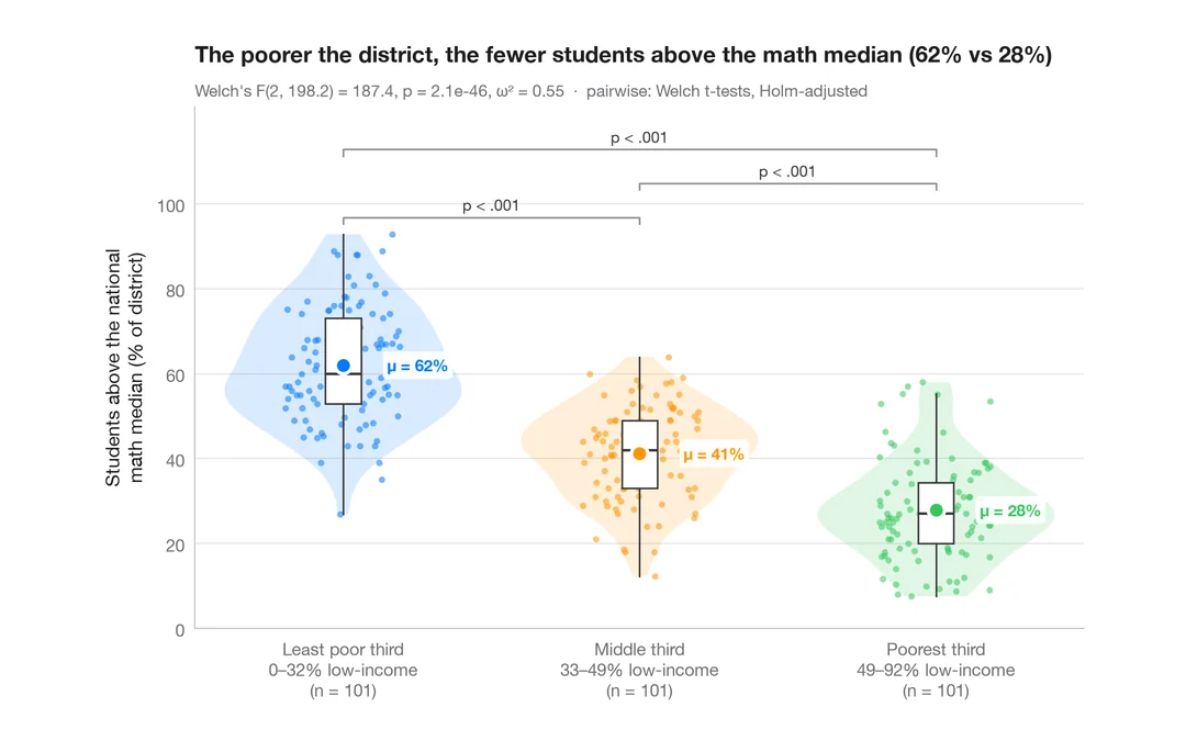
Between-groups comparison
Violin + box + points with Welch's ANOVA, effect size and pairwise tests.
ggstatsplot::ggbetweenstats()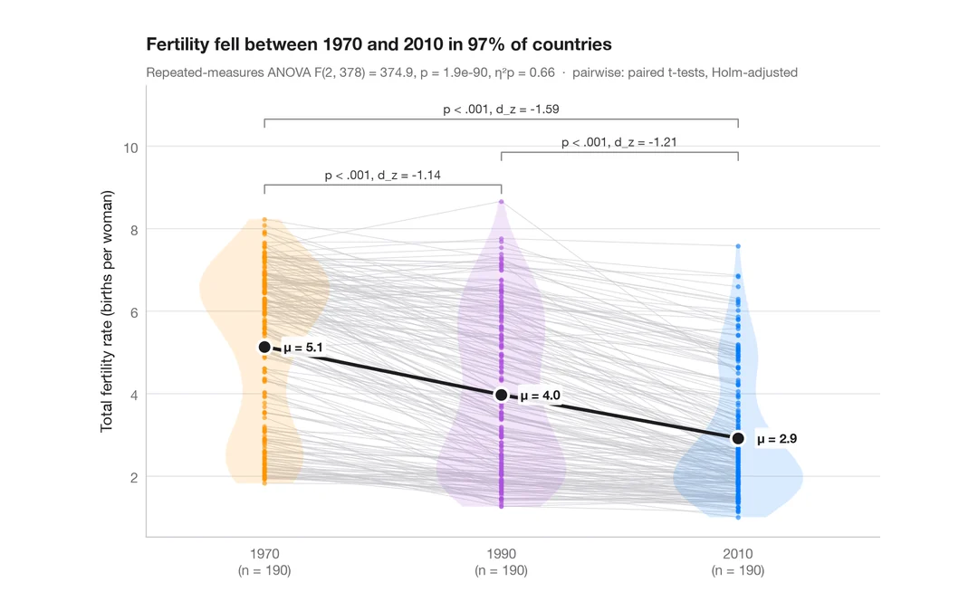
Within-subjects comparison
Repeated measures with one line per subject, means, rm-ANOVA and paired tests.
ggstatsplot::ggwithinstats()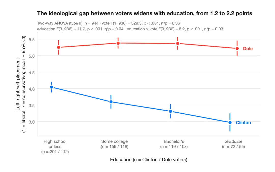
Interaction plot
Group means with 95% confidence intervals for two factors, with a two-way ANOVA.
ggpubr::ggline(add = "mean_ci") / ggstats