推定プロット
2群の生データに、平均値の差とそのブートストラップ 95% 信頼区間を添えます。
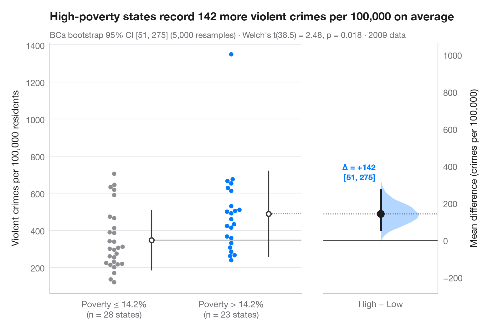
ガードナー・アルトマンの推定プロットは、p値ではなく効果量を中心に据えます。左の軸には両群のすべての観測値を示し、右側の浮いた軸はゼロが基準群の平均に一致するように配置されています。その軸上に、平均値の差のブートストラップ分布を半分のバイオリンとして描き、点推定値とその 95% 信頼区間を点と線で示しています。
データは statsmodels に同梱されている2009年の米国50州とコロンビア特別区です(sm.datasets.statecrime)。人口10万人あたりの暴力犯罪率を、貧困率が中央の州(14.2%)を上回る23州と、それ以下の28州とで比較しています。この比較は実験ではなく観察にもとづくもので、差の大きさを測るものであって、その原因を示すものではありません。95% 信頼区間は scipy.stats.bootstrap によるバイアス補正・加速(BCa)ブートストラップで、サブタイトルにはウェルチの t 検定(scipy.stats.ttest_ind)も示しています。各スウォームの横の縦線は群平均 ± 1 標準偏差を表し、スウォームは seaborn.swarmplot で描いています。1,300 を超える位置にある孤立した点はコロンビア特別区です。
コードおよび図中のテキストは英語です。
import matplotlib.pyplot as plt
import numpy as np
import seaborn as sns
import statsmodels.api as sm
from scipy import stats

# Data: violent crimes per 100,000 residents in 2009, by state poverty rate
df = sm.datasets.statecrime.load_pandas().data
cut = df.poverty.median()
df["group"] = np.where(df.poverty > cut, "High poverty", "Low poverty")
low = df.loc[df.group == "Low poverty", "violent"].to_numpy()
high = df.loc[df.group == "High poverty", "violent"].to_numpy()

# Mean difference with a BCa bootstrap 95% CI, and the bootstrap distribution
diff = lambda a, b, axis=-1: np.mean(b, axis=axis) - np.mean(a, axis=axis)
boot = stats.bootstrap((low, high), diff, n_resamples=5000, method="BCa",
                       random_state=np.random.default_rng(1))
lo, hi = boot.confidence_interval
delta = high.mean() - low.mean()
t = stats.ttest_ind(high, low, equal_var=False)

# Manual layout (the long subtitle would otherwise squeeze the panels apart)
fig, (ax, ax2) = plt.subplots(1, 2, figsize=(8, 5.2), width_ratios=[2.2, 1], layout="none")
fig.subplots_adjust(wspace=0.12)
palette = ["#8E8E93", "#007AFF"]
sns.swarmplot(data=df, x="group", y="violent", hue="group", palette=palette, size=5,
              order=["Low poverty", "High poverty"], hue_order=["Low poverty", "High poverty"],
              legend=False, ax=ax)
for i, d in enumerate([low, high]):            # mean ± SD as a gapped line beside the swarm
    m, s = d.mean(), d.std(ddof=1)
    ax.vlines(i + 0.32, m - s, m + s, color="#3A3A3C", lw=1.5)
    ax.scatter(i + 0.32, m, s=30, color="white", edgecolor="#3A3A3C", lw=1.5, zorder=3)
ax.set_xlabel("")
ax.set_ylabel("Violent crimes per 100,000 residents")
ax.set_xticks([0, 1], [f"Poverty ≤ {cut:.1f}%\n(n = {len(low)} states)",
                      f"Poverty > {cut:.1f}%\n(n = {len(high)} states)"])

# Floating difference axis: zero aligned with the low-poverty mean
ax.set_xlim(-0.55, 1.6)
ymin, ymax = ax.get_ylim()
ax2.set_ylim(ymin - low.mean(), ymax - low.mean())
ax2.axhline(0, color="#3A3A3C", lw=1)
ax2.axhline(delta, color="#3A3A3C", lw=1, ls=":")
ax.plot([0.32, 1.6], [low.mean()] * 2, color="#3A3A3C", lw=0.8)
ax.plot([1.32, 1.6], [high.mean()] * 2, color="#3A3A3C", lw=0.8, ls=":")
v = ax2.violinplot(boot.bootstrap_distribution, positions=[0], widths=0.8,
                   showextrema=False, side="high")
v["bodies"][0].set(facecolor="#007AFF", alpha=0.3, edgecolor="none")
ax2.vlines(0, lo, hi, color="#1D1D1F", lw=2.5)
ax2.scatter(0, delta, s=70, color="#1D1D1F", zorder=3)
ax2.annotate(f"Δ = {delta:+.0f}\n[{lo:.0f}, {hi:.0f}]", (0, hi), xytext=(-6, 8),
             textcoords="offset points", ha="right", va="bottom", fontsize=9.5,
             fontweight="semibold", color="#007AFF")
ax2.set_xlim(-0.6, 0.6)
ax2.set_xticks([0], ["High − Low"])
ax2.yaxis.tick_right(); ax2.yaxis.set_label_position("right")
ax2.spines[["left"]].set_visible(False); ax2.spines["right"].set_visible(True)
ax2.set_ylabel("Mean difference (crimes per 100,000)")
ax2.grid(False)

ax.set_title(f"High-poverty states record {delta:.0f} more violent crimes per 100,000 on average",
             pad=26)
ax.text(0, 1.02, f"BCa bootstrap 95% CI [{lo:.0f}, {hi:.0f}] (5,000 resamples) · "
        f"Welch's t({t.df:.1f}) = {t.statistic:.2f}, p = {t.pvalue:.3f} · 2009 data",
        transform=ax.transAxes, fontsize=9.5, color="#6E6E73")
plt.show()
図にはオプションの PyStatlas スタイル を使用しています。同じ見た目にするには plt.style.use("pystatlas.mplstyle") を追加してください。
データの出典
- US state crime and social indicators, 2009. U.S. Census Bureau. Statistical Abstract of the United States, state tables for 2009 (crime rates from the FBI Uniform Crime Reporting program). https://www.statsmodels.org/stable/datasets/generated/statecrime.html
Compiled for statsmodels (sm.datasets.statecrime); public domain. See the statsmodels page for each variable's table and footnotes.
これらの例は統計手法を説明するためのものです。図のタイトルは、この特定のデータ(多くは小規模で、古く、部分的な標本)で図が示す内容を述べたものであり、実質的な問いに対する著者の立場ではありません。解釈、背景、データの質については、ここに挙げた元の出典を参照してください。
引用方法
PyStatlas は Thierry Warin が作成・運営しています。研究や業務に役立った場合は、ぜひ引用してください。
Warin, T. (2026). Estimation plot. In PyStatlas: A Python Gallery of Statistical Graphics for the Social Sciences. https://warint.github.io/pystatlas/group-comparisons/estimation-plot/
@misc{warin2026statlas,
  author       = {Warin, Thierry},
  title        = {PyStatlas: A Python Gallery of Statistical Graphics for the Social Sciences},
  year         = {2026},
  howpublished = {\url{https://warint.github.io/pystatlas/}},
  note         = {Source code: https://github.com/warint/pystatlas}
}