估计图
两组原始数据,加上均值差及其自助法 95% 置信区间。
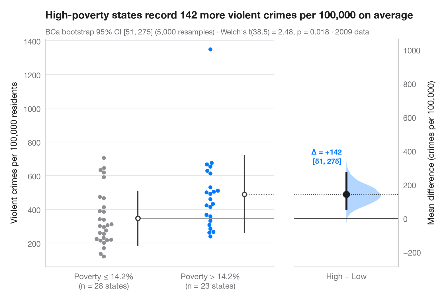
Gardner–Altman 估计图将效应量而非 p 值置于核心位置。左轴展示两组的全部观测值;右侧的浮动坐标轴经过对齐,使其零点正好位于参照组均值处。在这条轴上,均值差的自助法分布以半边小提琴图呈现,点估计及其 95% 置信区间分别以圆点和线段表示。
数据为 statsmodels 附带的 2009 年美国 50 个州加哥伦比亚特区(sm.datasets.statecrime):比较贫困率高于中位州(14.2%)的 23 个州与等于或低于该水平的 28 个州每 10 万居民的暴力犯罪率。该比较属于观察性研究而非实验:它衡量差距有多大,而不说明差距的成因。95% 置信区间来自 scipy.stats.bootstrap 的偏差校正加速(BCa)自助法,副标题另附 Welch t 检验(scipy.stats.ttest_ind);每组蜂群图旁的竖线表示组均值 ± 1 个标准差,蜂群图由 seaborn.swarmplot 绘制。高于 1,300 的那个孤立点是哥伦比亚特区。
代码及图中文字均为英文。
import matplotlib.pyplot as plt
import numpy as np
import seaborn as sns
import statsmodels.api as sm
from scipy import stats

# Data: violent crimes per 100,000 residents in 2009, by state poverty rate
df = sm.datasets.statecrime.load_pandas().data
cut = df.poverty.median()
df["group"] = np.where(df.poverty > cut, "High poverty", "Low poverty")
low = df.loc[df.group == "Low poverty", "violent"].to_numpy()
high = df.loc[df.group == "High poverty", "violent"].to_numpy()

# Mean difference with a BCa bootstrap 95% CI, and the bootstrap distribution
diff = lambda a, b, axis=-1: np.mean(b, axis=axis) - np.mean(a, axis=axis)
boot = stats.bootstrap((low, high), diff, n_resamples=5000, method="BCa",
                       random_state=np.random.default_rng(1))
lo, hi = boot.confidence_interval
delta = high.mean() - low.mean()
t = stats.ttest_ind(high, low, equal_var=False)

# Manual layout (the long subtitle would otherwise squeeze the panels apart)
fig, (ax, ax2) = plt.subplots(1, 2, figsize=(8, 5.2), width_ratios=[2.2, 1], layout="none")
fig.subplots_adjust(wspace=0.12)
palette = ["#8E8E93", "#007AFF"]
sns.swarmplot(data=df, x="group", y="violent", hue="group", palette=palette, size=5,
              order=["Low poverty", "High poverty"], hue_order=["Low poverty", "High poverty"],
              legend=False, ax=ax)
for i, d in enumerate([low, high]):            # mean ± SD as a gapped line beside the swarm
    m, s = d.mean(), d.std(ddof=1)
    ax.vlines(i + 0.32, m - s, m + s, color="#3A3A3C", lw=1.5)
    ax.scatter(i + 0.32, m, s=30, color="white", edgecolor="#3A3A3C", lw=1.5, zorder=3)
ax.set_xlabel("")
ax.set_ylabel("Violent crimes per 100,000 residents")
ax.set_xticks([0, 1], [f"Poverty ≤ {cut:.1f}%\n(n = {len(low)} states)",
                      f"Poverty > {cut:.1f}%\n(n = {len(high)} states)"])

# Floating difference axis: zero aligned with the low-poverty mean
ax.set_xlim(-0.55, 1.6)
ymin, ymax = ax.get_ylim()
ax2.set_ylim(ymin - low.mean(), ymax - low.mean())
ax2.axhline(0, color="#3A3A3C", lw=1)
ax2.axhline(delta, color="#3A3A3C", lw=1, ls=":")
ax.plot([0.32, 1.6], [low.mean()] * 2, color="#3A3A3C", lw=0.8)
ax.plot([1.32, 1.6], [high.mean()] * 2, color="#3A3A3C", lw=0.8, ls=":")
v = ax2.violinplot(boot.bootstrap_distribution, positions=[0], widths=0.8,
                   showextrema=False, side="high")
v["bodies"][0].set(facecolor="#007AFF", alpha=0.3, edgecolor="none")
ax2.vlines(0, lo, hi, color="#1D1D1F", lw=2.5)
ax2.scatter(0, delta, s=70, color="#1D1D1F", zorder=3)
ax2.annotate(f"Δ = {delta:+.0f}\n[{lo:.0f}, {hi:.0f}]", (0, hi), xytext=(-6, 8),
             textcoords="offset points", ha="right", va="bottom", fontsize=9.5,
             fontweight="semibold", color="#007AFF")
ax2.set_xlim(-0.6, 0.6)
ax2.set_xticks([0], ["High − Low"])
ax2.yaxis.tick_right(); ax2.yaxis.set_label_position("right")
ax2.spines[["left"]].set_visible(False); ax2.spines["right"].set_visible(True)
ax2.set_ylabel("Mean difference (crimes per 100,000)")
ax2.grid(False)

ax.set_title(f"High-poverty states record {delta:.0f} more violent crimes per 100,000 on average",
             pad=26)
ax.text(0, 1.02, f"BCa bootstrap 95% CI [{lo:.0f}, {hi:.0f}] (5,000 resamples) · "
        f"Welch's t({t.df:.1f}) = {t.statistic:.2f}, p = {t.pvalue:.3f} · 2009 data",
        transform=ax.transAxes, fontsize=9.5, color="#6E6E73")
plt.show()
图表使用了可选的 PyStatlas 样式:添加 plt.style.use("pystatlas.mplstyle") 即可完全还原其外观。
数据来源
- US state crime and social indicators, 2009. U.S. Census Bureau. Statistical Abstract of the United States, state tables for 2009 (crime rates from the FBI Uniform Crime Reporting program). https://www.statsmodels.org/stable/datasets/generated/statecrime.html
Compiled for statsmodels (sm.datasets.statecrime); public domain. See the statsmodels page for each variable's table and footnotes.
这些示例用于说明统计方法。图表标题描述的是该图在这些特定数据中呈现的内容——这些数据往往样本较小、年代较早或并不完整——而不是作者对实质问题的立场。关于解释、背景和数据质量,请以此处引用的原始来源为准。
如何引用
PyStatlas 由 Thierry Warin 创建并维护。如果它对你的工作有所帮助,敬请引用。
Warin, T. (2026). Estimation plot. In PyStatlas: A Python Gallery of Statistical Graphics for the Social Sciences. https://warint.github.io/pystatlas/group-comparisons/estimation-plot/
@misc{warin2026statlas,
  author       = {Warin, Thierry},
  title        = {PyStatlas: A Python Gallery of Statistical Graphics for the Social Sciences},
  year         = {2026},
  howpublished = {\url{https://warint.github.io/pystatlas/}},
  note         = {Source code: https://github.com/warint/pystatlas}
}