交互作用图
两个因素下各组均值及其 95% 置信区间,附双因素方差分析。
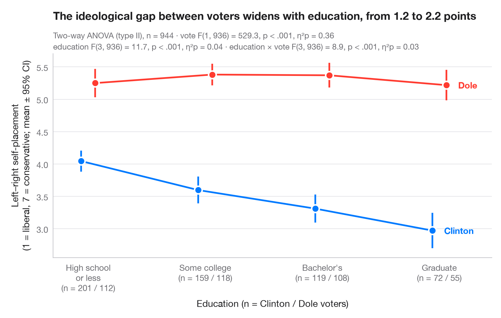
交互作用图展示两个因素每种组合下的结局均值:一个因素置于 x 轴,另一个以彩色、略微错开的折线表示。每个均值都带有 95% 置信区间。折线平行意味着两个因素独立起作用;折线趋近、发散或交叉则提示存在交互作用。
数据为 statsmodels 附带的 1996 年美国全国选举研究中的 944 名选民(sm.datasets.anes96):他们在 7 点自由–保守量表上的自我定位(1 = 极端自由,7 = 极端保守),按受教育程度(将调查的七个编码归并为四个等级)和总统选举投票对象(克林顿或多尔)分组。双因素方差分析(II 型平方和)由 statsmodels.formula.api.ols 和 statsmodels.stats.anova.anova_lm 计算,并为每一项给出偏 η²;置信区间基于 t 分布。
代码及图中文字均为英文。
import matplotlib.pyplot as plt
import numpy as np
import pandas as pd
import statsmodels.api as sm
import statsmodels.formula.api as smf
from scipy import stats
from statsmodels.stats.anova import anova_lm

# Data: left–right self-placement (1–7) by education level and presidential vote
df = sm.datasets.anes96.load_pandas().data
classes = ["High school\nor less", "Some college", "Bachelor's", "Graduate"]
df["educ_level"] = pd.cut(df.educ, [0, 3, 5, 6, 7], labels=classes)  # survey codes 1–3, 4–5, 6, 7
df["voter"] = df.vote.map({0: "Clinton", 1: "Dole"})

# Two-way ANOVA with interaction (type II) + partial eta squared
aov = anova_lm(smf.ols("selfLR ~ C(educ_level) * C(voter)", data=df).fit(), typ=2)
ss_res = aov.loc["Residual", "sum_sq"]
aov["eta_p"] = aov.sum_sq / (aov.sum_sq + ss_res)
df_res = int(aov.loc["Residual", "df"])

# Means and t-based 95% CIs per cell
cells = df.groupby(["voter", "educ_level"], observed=True).selfLR.agg(["mean", "sem", "count"])
cells["half"] = cells["sem"] * stats.t.ppf(0.975, cells["count"] - 1)

fig, ax = plt.subplots(figsize=(8, 5))
x = np.arange(len(classes))
for (voter, c, dx) in [("Clinton", "#007AFF", -0.06), ("Dole", "#FF3B30", 0.06)]:
    m = cells.loc[voter].reindex(classes)
    ax.errorbar(x + dx, m["mean"], yerr=m["half"], color=c, lw=2, capsize=0,
                elinewidth=2, marker="o", ms=9, mec="white", mew=1.8, label=voter)
    ax.annotate(voter, (x[-1] + dx, m["mean"].iloc[-1]), xytext=(14, 0),
                textcoords="offset points", va="center", fontsize=10.5,
                fontweight="semibold", color=c)

# Cell sizes under the axis labels
n = cells["count"].unstack(0).reindex(classes)
ax.set_xticks(x, [f"{k}\n(n = {n.loc[k, 'Clinton']} / {n.loc[k, 'Dole']})" for k in classes])
ax.set_xlim(-0.3, len(classes) - 0.55)
ax.set_xlabel("Education (n = Clinton / Dole voters)")
ax.set_ylabel("Left–right self-placement\n(1 = liberal, 7 = conservative; mean ± 95% CI)")

# One "F(df1, df2) = …, p …, η²p = …" string per ANOVA term
stat = {}
for term, label in [("C(educ_level)", "education"), ("C(voter)", "vote"), ("C(educ_level):C(voter)", "education × vote")]:
    r = aov.loc[term]
    pval = "< .001" if r["PR(>F)"] < .001 else f"= {r['PR(>F)']:.2f}"
    stat[label] = f"{label} F({r.df:.0f}, {df_res}) = {r.F:.1f}, p {pval}, η²p = {r.eta_p:.2f}"

gap = cells.loc["Dole", "mean"] - cells.loc["Clinton", "mean"]
ax.set_title(f"The ideological gap between voters widens with education, "
             f"from {gap.iloc[0]:.1f} to {gap.iloc[-1]:.1f} points", pad=40)
ax.text(0, 1.075, f"Two-way ANOVA (type II), n = {len(df)} · {stat['vote']}",
        transform=ax.transAxes, fontsize=9.5, color="#6E6E73")
ax.text(0, 1.02, f"{stat['education']} · {stat['education × vote']}", transform=ax.transAxes,
        fontsize=9.5, color="#6E6E73")
plt.show()
图表使用了可选的 PyStatlas 样式:添加 plt.style.use("pystatlas.mplstyle") 即可完全还原其外观。
数据来源
- American National Election Study, 1996. Rosenstone, S. J., Kinder, D. R., Miller, W. E., & the National Election Studies. (2016). ANES 1996 Time Series Study (ICPSR 6896; Version 6) [Data set]. Inter-university Consortium for Political and Social Research. https://doi.org/10.3886/ICPSR06896.v6
Subset of 944 respondents distributed with statsmodels (sm.datasets.anes96); public domain.
这些示例用于说明统计方法。图表标题描述的是该图在这些特定数据中呈现的内容——这些数据往往样本较小、年代较早或并不完整——而不是作者对实质问题的立场。关于解释、背景和数据质量,请以此处引用的原始来源为准。
如何引用
PyStatlas 由 Thierry Warin 创建并维护。如果它对你的工作有所帮助,敬请引用。
Warin, T. (2026). Interaction plot. In PyStatlas: A Python Gallery of Statistical Graphics for the Social Sciences. https://warint.github.io/pystatlas/group-comparisons/means-with-ci/
@misc{warin2026statlas,
  author       = {Warin, Thierry},
  title        = {PyStatlas: A Python Gallery of Statistical Graphics for the Social Sciences},
  year         = {2026},
  howpublished = {\url{https://warint.github.io/pystatlas/}},
  note         = {Source code: https://github.com/warint/pystatlas}
}