组间比较
小提琴图 + 箱线图 + 散点,附 Welch 方差分析、效应量和两两检验。
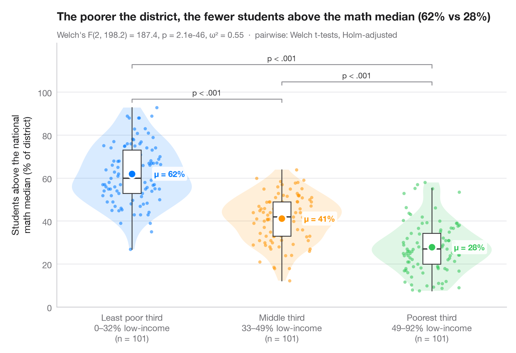
ggbetweenstats() 的 Python 版本:展示每一个观测值,外面包裹小提琴图(分布)和细长的箱线图(四分位数),并突出显示各组均值。副标题报告 Welch 单因素方差分析(对方差不齐稳健),以及作为效应量的 ω²;括号标注经 Holm 校正的两两 Welch t 检验结果。
数据为 statsmodels 附带的 1998 年 STAR 考试中加利福尼亚州的 303 个学区(sm.datasets.star98)。结局变量是数学成绩高于全国中位数的学生所占比例 NABOVE / (NABOVE + NBELOW),分组依据是学区内低收入家庭学生百分比(LOWINC)的三分位数,用 pandas.qcut 切分为各含 101 个学区的三组。
代码及图中文字均为英文。
from itertools import combinations

import matplotlib.pyplot as plt
import numpy as np
import pandas as pd
import statsmodels.api as sm
from scipy import stats
from statsmodels.stats.multitest import multipletests
from statsmodels.stats.oneway import anova_oneway

# Data: % of students above the national math median, by district low-income tercile
df = sm.datasets.star98.load_pandas().data
df["above"] = 100 * df.NABOVE / (df.NABOVE + df.NBELOW)
groups = ["Least poor third", "Middle third", "Poorest third"]
df["poverty"] = pd.qcut(df.LOWINC, 3, labels=groups)
data = [df.loc[df.poverty == g, "above"].to_numpy() for g in groups]
palette = ["#007AFF", "#FF9500", "#34C759"]

# Welch's ANOVA + omega squared
res = anova_oneway(data, use_var="unequal")
k, n = len(data), sum(len(d) for d in data)
omega2 = (res.statistic - 1) * (k - 1) / ((res.statistic - 1) * (k - 1) + n)

# Pairwise Welch t-tests, Holm-corrected
pairs = list(combinations(range(k), 2))
raw_p = [stats.ttest_ind(data[i], data[j], equal_var=False).pvalue for i, j in pairs]
adj_p = multipletests(raw_p, method="holm")[1]

fig, ax = plt.subplots(figsize=(8, 5.4))
rng = np.random.default_rng(1)
for i, (d, c) in enumerate(zip(data, palette)):
    v = ax.violinplot(d, positions=[i], widths=0.8, showextrema=False)
    for body in v["bodies"]:
        body.set(facecolor=c, alpha=0.15, edgecolor="none")
    ax.boxplot(d, positions=[i], widths=0.12, showfliers=False, patch_artist=True,
               boxprops=dict(facecolor="white", edgecolor="#3A3A3C", lw=1),
               medianprops=dict(color="#3A3A3C", lw=1.5),
               whiskerprops=dict(color="#3A3A3C"), capprops=dict(visible=False))
    ax.scatter(i + rng.uniform(-0.22, 0.22, len(d)) * 0.9, d, s=14, color=c, alpha=0.55, lw=0)
    ax.scatter(i, d.mean(), s=90, color=c, edgecolor="white", lw=2, zorder=5)
    ax.annotate(f"μ = {d.mean():.0f}%", (i + 0.09, d.mean()), xytext=(10, 0), textcoords="offset points",
                va="center", bbox=dict(boxstyle="round,pad=0.25", fc="white", ec="none", alpha=0.9), fontsize=9.5, fontweight="semibold", color=c)

# Significance brackets
top, step = max(map(np.max, data)), 8
for h, ((i, j), p) in enumerate(sorted(zip(pairs, adj_p), key=lambda t: t[0][1] - t[0][0])):
    y = top + 4 + h * step
    ax.plot([i, i, j, j], [y - 1.5, y, y, y - 1.5], color="#8E8E93", lw=1)
    label = "p < .001" if p < 0.001 else f"p = {p:.3f}"
    ax.text((i + j) / 2, y + 0.8, label, ha="center", va="bottom", fontsize=9, color="#3A3A3C")

lowinc = df.groupby("poverty", observed=True).LOWINC.agg(["min", "max"])
ax.set_xticks(range(k), [f"{g}\n{lowinc.loc[g, 'min']:.0f}–{lowinc.loc[g, 'max']:.0f}% low-income"
                         f"\n(n = {len(d)})" for g, d in zip(groups, data)])
ax.set_ylabel("Students above the national\nmath median (% of district)")
ax.set_ylim(top=top + 4 + len(pairs) * step + 2)
ax.set_yticks(range(0, 101, 20))
ax.set_title(f"The poorer the district, the fewer students above the math median "
             f"({data[0].mean():.0f}% vs {data[-1].mean():.0f}%)", pad=26)
ax.text(0, 1.02, f"Welch's F({res.df_num:.0f}, {res.df_denom:.1f}) = {res.statistic:.1f}, "
        f"p = {res.pvalue:.1e}, ω² = {omega2:.2f}  ·  pairwise: Welch t-tests, Holm-adjusted",
        transform=ax.transAxes, fontsize=9.5, color="#6E6E73")
plt.show()
图表使用了可选的 PyStatlas 样式:添加 plt.style.use("pystatlas.mplstyle") 即可完全还原其外观。
数据来源
- California STAR test results, 1998 (303 school districts). Gill, J. (2001). Generalized Linear Models: A Unified Approach (Quantitative Applications in the Social Sciences, No. 134). Sage. https://www.statsmodels.org/stable/datasets/generated/star98.html
Original data from the California Department of Education's Standardized Testing and Reporting (STAR) program, 1998. Subset distributed with statsmodels (sm.datasets.star98) with the author's permission.
这些示例用于说明统计方法。图表标题描述的是该图在这些特定数据中呈现的内容——这些数据往往样本较小、年代较早或并不完整——而不是作者对实质问题的立场。关于解释、背景和数据质量,请以此处引用的原始来源为准。
如何引用
PyStatlas 由 Thierry Warin 创建并维护。如果它对你的工作有所帮助,敬请引用。
Warin, T. (2026). Between-groups comparison. In PyStatlas: A Python Gallery of Statistical Graphics for the Social Sciences. https://warint.github.io/pystatlas/group-comparisons/between-groups-violin/
@misc{warin2026statlas,
  author       = {Warin, Thierry},
  title        = {PyStatlas: A Python Gallery of Statistical Graphics for the Social Sciences},
  year         = {2026},
  howpublished = {\url{https://warint.github.io/pystatlas/}},
  note         = {Source code: https://github.com/warint/pystatlas}
}