Comparaison entre groupes
Violon, boîte et points avec ANOVA de Welch, taille d'effet et tests deux à deux.
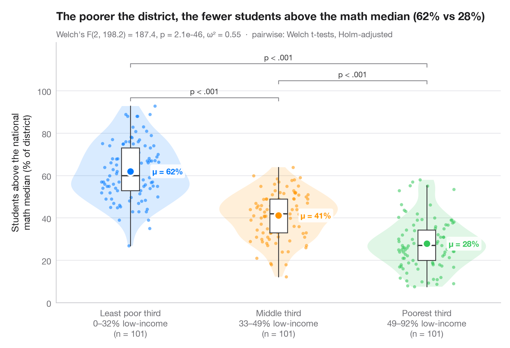
L'équivalent Python de ggbetweenstats() : chaque observation est affichée, enveloppée d'un violon (distribution) et d'une fine boîte (quartiles), avec la moyenne du groupe mise en évidence. Le sous-titre rapporte l'ANOVA à un facteur de Welch — robuste à l'inégalité des variances — avec ω² comme taille d'effet, et des crochets indiquent les tests t de Welch deux à deux corrigés selon Holm.
Les données sont les 303 districts scolaires californiens du test STAR de 1998 fournis avec statsmodels (sm.datasets.star98). La variable étudiée est la part des élèves qui obtiennent un score supérieur à la médiane nationale en mathématiques, NABOVE / (NABOVE + NBELOW), et les groupes sont les terciles du pourcentage d'élèves à faible revenu dans le district (LOWINC), découpés avec pandas.qcut en trois groupes de 101 districts.
Le code et le texte à l'intérieur des figures sont en anglais.
from itertools import combinations

import matplotlib.pyplot as plt
import numpy as np
import pandas as pd
import statsmodels.api as sm
from scipy import stats
from statsmodels.stats.multitest import multipletests
from statsmodels.stats.oneway import anova_oneway

# Data: % of students above the national math median, by district low-income tercile
df = sm.datasets.star98.load_pandas().data
df["above"] = 100 * df.NABOVE / (df.NABOVE + df.NBELOW)
groups = ["Least poor third", "Middle third", "Poorest third"]
df["poverty"] = pd.qcut(df.LOWINC, 3, labels=groups)
data = [df.loc[df.poverty == g, "above"].to_numpy() for g in groups]
palette = ["#007AFF", "#FF9500", "#34C759"]

# Welch's ANOVA + omega squared
res = anova_oneway(data, use_var="unequal")
k, n = len(data), sum(len(d) for d in data)
omega2 = (res.statistic - 1) * (k - 1) / ((res.statistic - 1) * (k - 1) + n)

# Pairwise Welch t-tests, Holm-corrected
pairs = list(combinations(range(k), 2))
raw_p = [stats.ttest_ind(data[i], data[j], equal_var=False).pvalue for i, j in pairs]
adj_p = multipletests(raw_p, method="holm")[1]

fig, ax = plt.subplots(figsize=(8, 5.4))
rng = np.random.default_rng(1)
for i, (d, c) in enumerate(zip(data, palette)):
    v = ax.violinplot(d, positions=[i], widths=0.8, showextrema=False)
    for body in v["bodies"]:
        body.set(facecolor=c, alpha=0.15, edgecolor="none")
    ax.boxplot(d, positions=[i], widths=0.12, showfliers=False, patch_artist=True,
               boxprops=dict(facecolor="white", edgecolor="#3A3A3C", lw=1),
               medianprops=dict(color="#3A3A3C", lw=1.5),
               whiskerprops=dict(color="#3A3A3C"), capprops=dict(visible=False))
    ax.scatter(i + rng.uniform(-0.22, 0.22, len(d)) * 0.9, d, s=14, color=c, alpha=0.55, lw=0)
    ax.scatter(i, d.mean(), s=90, color=c, edgecolor="white", lw=2, zorder=5)
    ax.annotate(f"μ = {d.mean():.0f}%", (i + 0.09, d.mean()), xytext=(10, 0), textcoords="offset points",
                va="center", bbox=dict(boxstyle="round,pad=0.25", fc="white", ec="none", alpha=0.9), fontsize=9.5, fontweight="semibold", color=c)

# Significance brackets
top, step = max(map(np.max, data)), 8
for h, ((i, j), p) in enumerate(sorted(zip(pairs, adj_p), key=lambda t: t[0][1] - t[0][0])):
    y = top + 4 + h * step
    ax.plot([i, i, j, j], [y - 1.5, y, y, y - 1.5], color="#8E8E93", lw=1)
    label = "p < .001" if p < 0.001 else f"p = {p:.3f}"
    ax.text((i + j) / 2, y + 0.8, label, ha="center", va="bottom", fontsize=9, color="#3A3A3C")

lowinc = df.groupby("poverty", observed=True).LOWINC.agg(["min", "max"])
ax.set_xticks(range(k), [f"{g}\n{lowinc.loc[g, 'min']:.0f}–{lowinc.loc[g, 'max']:.0f}% low-income"
                         f"\n(n = {len(d)})" for g, d in zip(groups, data)])
ax.set_ylabel("Students above the national\nmath median (% of district)")
ax.set_ylim(top=top + 4 + len(pairs) * step + 2)
ax.set_yticks(range(0, 101, 20))
ax.set_title(f"The poorer the district, the fewer students above the math median "
             f"({data[0].mean():.0f}% vs {data[-1].mean():.0f}%)", pad=26)
ax.text(0, 1.02, f"Welch's F({res.df_num:.0f}, {res.df_denom:.1f}) = {res.statistic:.1f}, "
        f"p = {res.pvalue:.1e}, ω² = {omega2:.2f}  ·  pairwise: Welch t-tests, Holm-adjusted",
        transform=ax.transAxes, fontsize=9.5, color="#6E6E73")
plt.show()
Les figures utilisent le style PyStatlas (facultatif) : ajoutez plt.style.use("pystatlas.mplstyle") pour obtenir exactement le même rendu.
Source des données
- California STAR test results, 1998 (303 school districts). Gill, J. (2001). Generalized Linear Models: A Unified Approach (Quantitative Applications in the Social Sciences, No. 134). Sage. https://www.statsmodels.org/stable/datasets/generated/star98.html
Original data from the California Department of Education's Standardized Testing and Reporting (STAR) program, 1998. Subset distributed with statsmodels (sm.datasets.star98) with the author's permission.
Les exemples illustrent des méthodes statistiques. Leurs titres décrivent ce que chaque figure montre dans ces données précises — souvent un échantillon restreint, daté ou partiel —, et non la position de l'auteur sur la question de fond. Pour l'interprétation, le contexte et la qualité des données, reportez-vous aux sources originales citées ici.
Comment citer
PyStatlas est créé et maintenu par Thierry Warin. S'il vous a été utile dans vos travaux, merci de le citer.
Warin, T. (2026). Between-groups comparison. In PyStatlas: A Python Gallery of Statistical Graphics for the Social Sciences. https://warint.github.io/pystatlas/group-comparisons/between-groups-violin/
@misc{warin2026statlas,
  author       = {Warin, Thierry},
  title        = {PyStatlas: A Python Gallery of Statistical Graphics for the Social Sciences},
  year         = {2026},
  howpublished = {\url{https://warint.github.io/pystatlas/}},
  note         = {Source code: https://github.com/warint/pystatlas}
}Plus dans Comparaisons de groupes
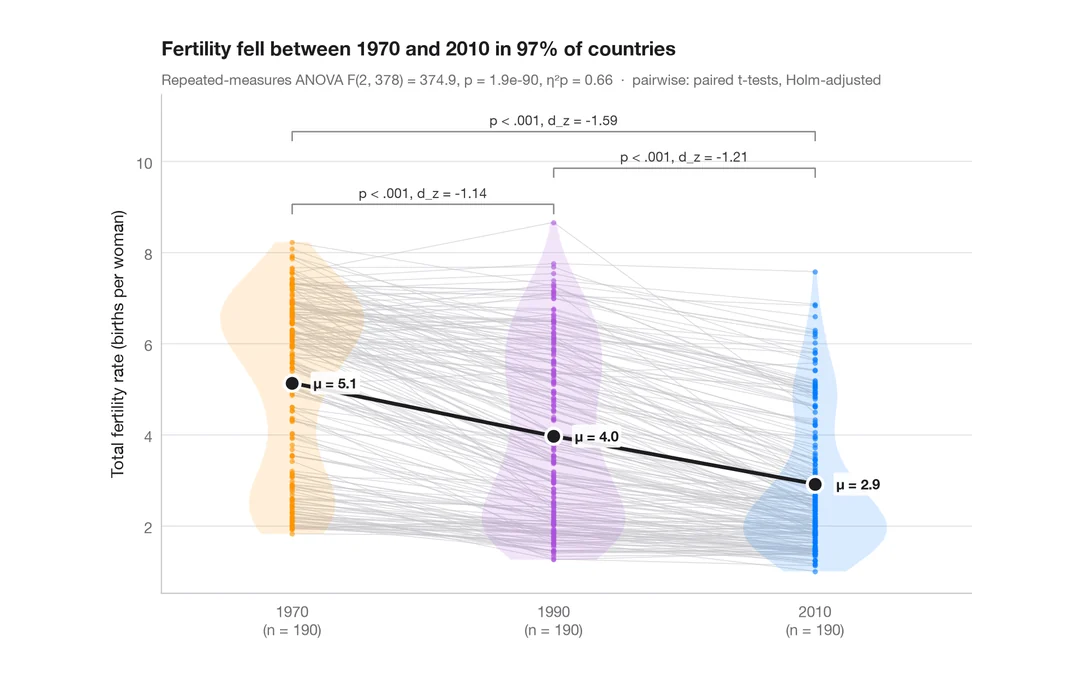
Comparaison intra-sujets
Mesures répétées avec une ligne par sujet, moyennes, ANOVA à mesures répétées et tests appariés.
ggstatsplot::ggwithinstats()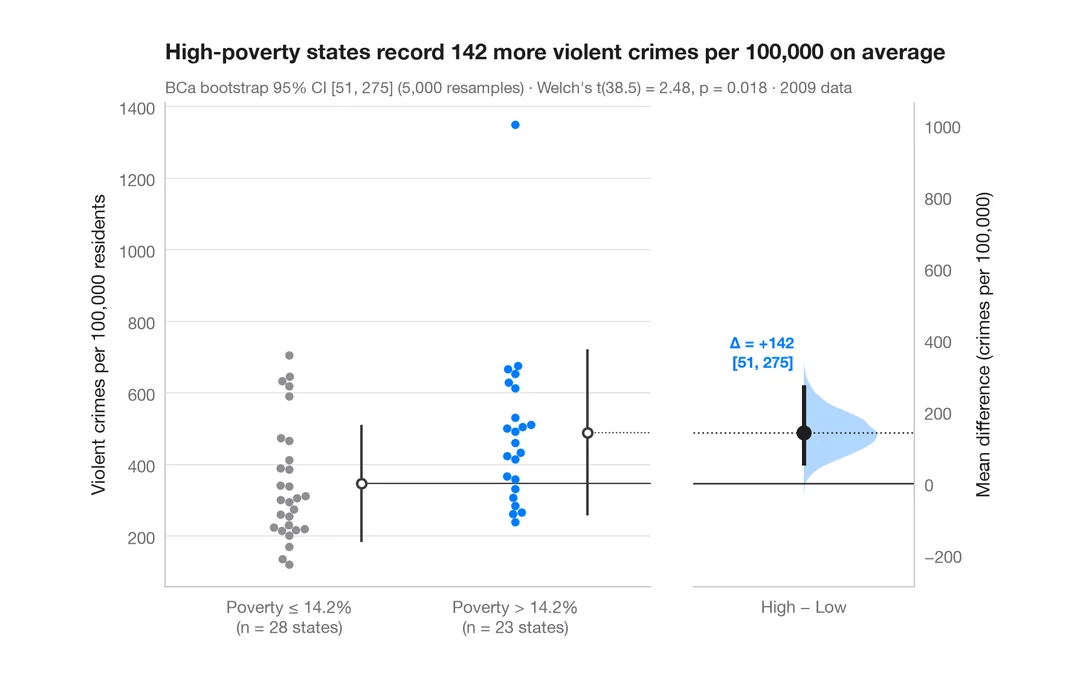
Graphique d'estimation
Données brutes de deux groupes, avec la différence de moyennes et son IC à 95 % par bootstrap.
dabestr::dabest() + plot()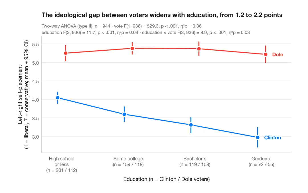
Graphique d'interaction
Moyennes de groupes avec intervalles de confiance à 95 % pour deux facteurs, avec ANOVA à deux facteurs.
ggpubr::ggline(add = "mean_ci") / ggstats