被験者内比較
被験者ごとの線、平均、反復測定分散分析、対応のある検定で反復測定データを示します。
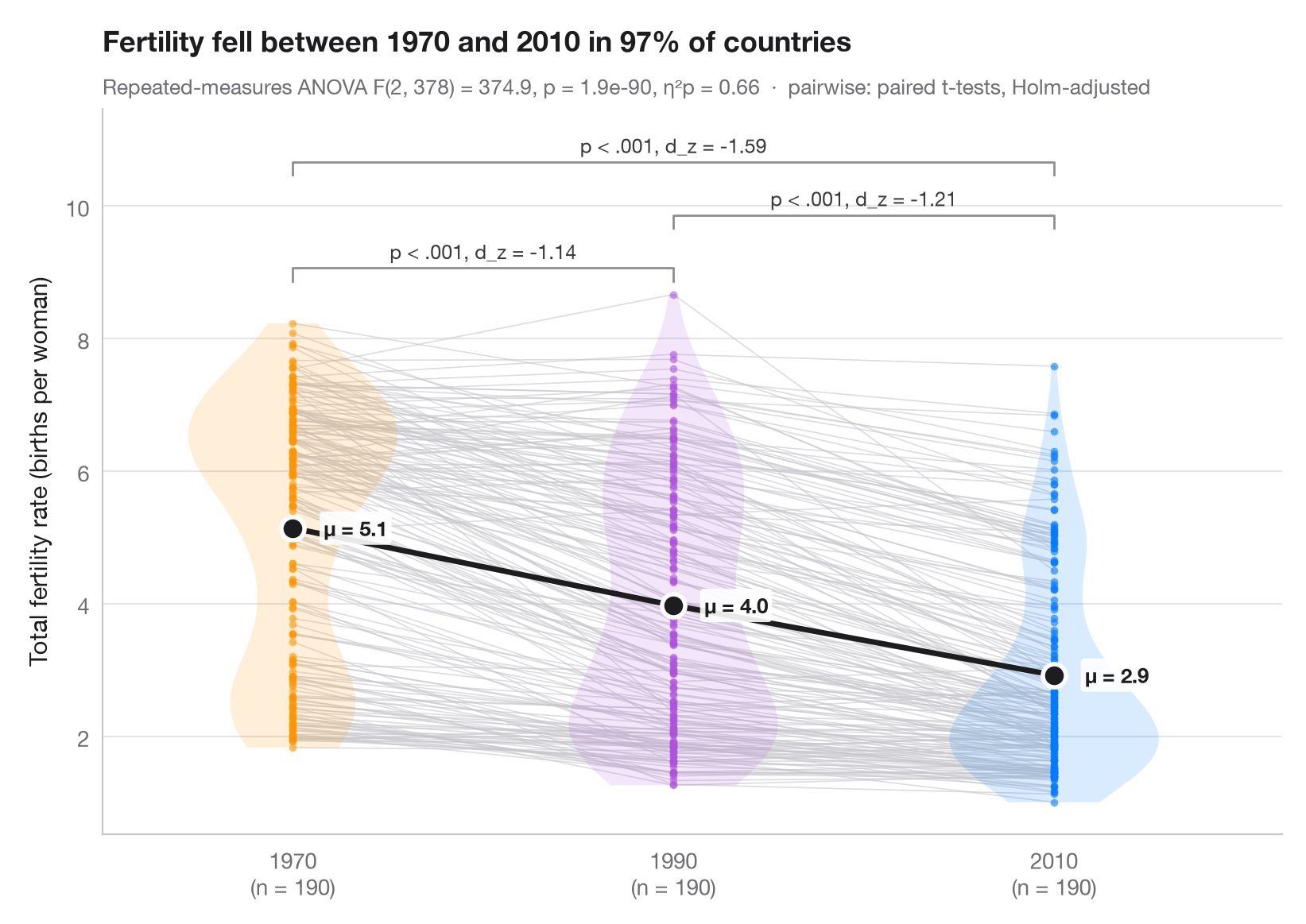
同じ単位をすべての条件で測定した場合、注目すべき変動は各単位の 内部 にあります。細い灰色の線が各国の測定値を結ぶので、ほぼすべての国が同じ方向に変化しているかどうかがわかります。バイオリンは年ごとの分布を示し、大きな点(濃い色の線で結んだもの)が年ごとの平均です。
データは statsmodels に同梱されている世界銀行の合計特殊出生率(女性1人あたりの出生数、sm.datasets.fertility)で、1970、1990、2010年のすべてに値がある190か国(地域集計値は除外)を対象としているため、各国が3回測定されていることになります。サブタイトルには一元配置の反復測定分散分析(statsmodels.stats.anova.AnovaRM)の結果を偏 η² とともに示し、括弧はホルム法で補正した対応のある t 検定(scipy.stats.ttest_rel)の結果をコーエンの d_z(負の値=出生率の低下)とともに表しています。
コードおよび図中のテキストは英語です。
from itertools import combinations

import matplotlib.pyplot as plt
import numpy as np
import pandas as pd
import statsmodels.api as sm
from scipy import stats
from statsmodels.stats.anova import AnovaRM
from statsmodels.stats.multitest import multipletests

# Data: fertility of the same countries in 1970, 1990 and 2010 (births per woman)
wb = sm.datasets.fertility.load_pandas().data
wb = wb[~wb["Country Name"].str.contains("classification|income levels|members|small states")]  # 5 aggregates
conditions = ["1970", "1990", "2010"]
wide = wb[conditions].dropna().reset_index(drop=True)
n = len(wide)
long = wide.rename_axis("id").reset_index().melt("id", var_name="condition", value_name="tfr")

# Repeated-measures ANOVA + partial eta squared
aov = AnovaRM(long, "tfr", "id", within=["condition"]).fit().anova_table.iloc[0]
eta_p = aov["F Value"] * aov["Num DF"] / (aov["F Value"] * aov["Num DF"] + aov["Den DF"])

# Pairwise paired t-tests (Holm) with Cohen's d_z
pairs = list(combinations(range(3), 2))
tests = [stats.ttest_rel(wide.iloc[:, j], wide.iloc[:, i]) for i, j in pairs]
adj_p = multipletests([t.pvalue for t in tests], method="holm")[1]
dz = [(wide.iloc[:, j] - wide.iloc[:, i]).mean() / (wide.iloc[:, j] - wide.iloc[:, i]).std()
      for i, j in pairs]

fig, ax = plt.subplots(figsize=(8, 5.6))
palette = ["#FF9500", "#AF52DE", "#007AFF"]
x = np.arange(3)
for _, row in wide.iterrows():                      # one line per subject
    ax.plot(x, row.values, color="#C7C7CC", lw=0.6, alpha=0.6, zorder=1)
for i, c in enumerate(palette):
    v = ax.violinplot(wide.iloc[:, i], positions=[i], widths=0.55, showextrema=False)
    v["bodies"][0].set(facecolor=c, alpha=0.15, edgecolor="none")
    ax.scatter(np.full(n, i), wide.iloc[:, i], s=12, color=c, alpha=0.6, lw=0, zorder=2)
means = wide.mean()
ax.plot(x, means, color="#1D1D1F", lw=2.5, zorder=3)
ax.scatter(x, means, s=110, color="#1D1D1F", edgecolor="white", lw=2, zorder=4)
for i, m in enumerate(means):
    ax.annotate(f"μ = {m:.1f}", (i, m), xytext=(14, 0), textcoords="offset points", va="center",
                fontsize=9.5, fontweight="semibold", color="#1D1D1F",
                bbox=dict(boxstyle="round,pad=0.2", fc="white", ec="none", alpha=0.9), zorder=5)

# Significance brackets
top, step = wide.values.max() + 0.4, 0.8
for h, ((i, j), p, d) in enumerate(sorted(zip(pairs, adj_p, dz), key=lambda t: t[0][1] - t[0][0])):
    y = top + h * step
    ax.plot([i, i, j, j], [y - 0.2, y, y, y - 0.2], color="#8E8E93", lw=1)
    label = "p < .001" if p < 0.001 else f"p = {p:.3f}"
    ax.text((i + j) / 2, y + 0.07, f"{label}, d_z = {d:.2f}", ha="center", va="bottom",
            fontsize=9, color="#3A3A3C")

ax.set_xticks(x, [f"{c}\n(n = {n})" for c in conditions])
ax.set_xlim(-0.5, 2.6)
ax.set_ylim(top=top + 3 * step)
ax.set_ylabel("Total fertility rate (births per woman)")
fell = (wide["2010"] < wide["1970"]).mean()
ax.set_title(f"Fertility fell between 1970 and 2010 in {fell:.0%} of countries", pad=26)
ax.text(0, 1.02, f"Repeated-measures ANOVA F({aov['Num DF']:.0f}, {aov['Den DF']:.0f}) = "
        f"{aov['F Value']:.1f}, p = {aov['Pr > F']:.1e}, η²p = {eta_p:.2f}  ·  "
        "pairwise: paired t-tests, Holm-adjusted", transform=ax.transAxes,
        fontsize=9.5, color="#6E6E73")
plt.show()
図にはオプションの PyStatlas スタイル を使用しています。同じ見た目にするには plt.style.use("pystatlas.mplstyle") を追加してください。
データの出典
- World Bank fertility rates by country, 1960–2013. World Bank. Fertility rate, total (births per woman), indicator SP.DYN.TFRT.IN. World Development Indicators. https://data.worldbank.org/indicator/SP.DYN.TFRT.IN
Primary sources: UN Population Division, UN Statistical Division, national statistical offices, Eurostat and others. Distributed with statsmodels (sm.datasets.fertility) under the World Bank terms of use.
これらの例は統計手法を説明するためのものです。図のタイトルは、この特定のデータ(多くは小規模で、古く、部分的な標本)で図が示す内容を述べたものであり、実質的な問いに対する著者の立場ではありません。解釈、背景、データの質については、ここに挙げた元の出典を参照してください。
引用方法
PyStatlas は Thierry Warin が作成・運営しています。研究や業務に役立った場合は、ぜひ引用してください。
Warin, T. (2026). Within-subjects comparison. In PyStatlas: A Python Gallery of Statistical Graphics for the Social Sciences. https://warint.github.io/pystatlas/group-comparisons/within-subjects/
@misc{warin2026statlas,
  author       = {Warin, Thierry},
  title        = {PyStatlas: A Python Gallery of Statistical Graphics for the Social Sciences},
  year         = {2026},
  howpublished = {\url{https://warint.github.io/pystatlas/}},
  note         = {Source code: https://github.com/warint/pystatlas}
}