ACF and PACF

Warin, Thierry

Autocorrelation and partial autocorrelation of US quarterly unemployment, as lollipops with 95% significance bands.

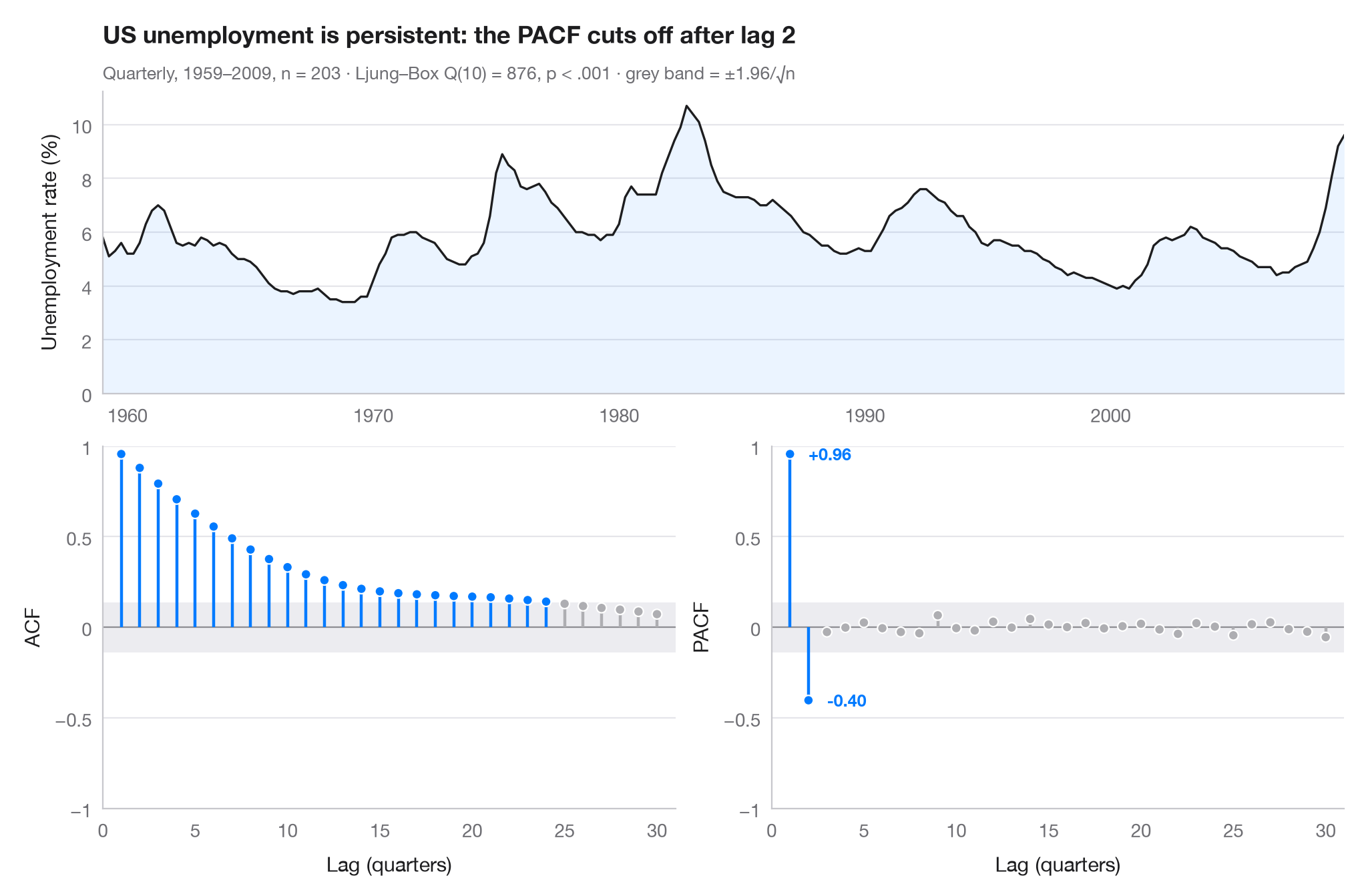
The autocorrelation function (ACF) measures how strongly a series correlates with itself k steps earlier; the partial autocorrelation (PACF) does the same after removing the effect of the shorter lags in between. Stems that leave the grey band (±1.96/√n) are larger than white noise would produce. Together the two panels suggest a model: here the ACF decays slowly over several years — high unemployment today means high unemployment next year — while the PACF cuts off after two lags, the signature of an AR(2) process.

Data are the US civilian unemployment rate, quarterly 1959Q1–2009Q3 (203 quarters), from the macroeconomic dataset bundled with statsmodels (sm.datasets.macrodata, column unemp). Correlations come from statsmodels.tsa.stattools.acf and pacf, and the subtitle reports a Ljung–Box test of no autocorrelation.

acf-pacf.py · 47 lines

Download GitHub

import matplotlib.pyplot as plt
import numpy as np
import statsmodels.api as sm
from statsmodels.stats.diagnostic import acorr_ljungbox
from statsmodels.tsa.stattools import acf, pacf

# Data: US unemployment rate, quarterly
df = sm.datasets.macrodata.load_pandas().data
y = df.set_index(df.year + (df.quarter - 1) / 4)["unemp"]
n, nlags = len(y), 30
band = 1.96 / np.sqrt(n)
lb = acorr_ljungbox(y, lags=[10]).iloc[0]

fig = plt.figure(figsize=(10, 6.5))
gs = fig.add_gridspec(2, 2, height_ratios=[1, 1.2])
ax_ts = fig.add_subplot(gs[0, :])
axes = [fig.add_subplot(gs[1, 0]), fig.add_subplot(gs[1, 1])]

# Top: the series itself
ax_ts.plot(y.index, y, color="#1D1D1F", lw=1.2)
ax_ts.fill_between(y.index, y, color="#007AFF", alpha=0.08, lw=0)
ax_ts.set(ylabel="Unemployment rate (%)", xlim=(y.index[0], y.index[-1]), ylim=(0, None))

# Bottom: ACF and PACF as lollipops with the white-noise band
values = [acf(y, nlags=nlags)[1:], pacf(y, nlags=nlags, method="ywm")[1:]]
for ax, v, name in zip(axes, values, ["ACF", "PACF"]):
    lags = np.arange(1, nlags + 1)
    sig = np.abs(v) > band
    colors = np.where(sig, "#007AFF", "#AEAEB2")
    ax.axhspan(-band, band, color="#E5E5EA", alpha=0.7, lw=0)
    ax.axhline(0, color="#8E8E93", lw=0.8)
    ax.vlines(lags, 0, v, color=colors, lw=1.6)
    ax.scatter(lags, v, s=28, color=colors, edgecolor="white", lw=0.8, zorder=3)
    ax.set(xlabel="Lag (quarters)", ylabel=name, ylim=(-1, 1), xlim=(0, nlags + 1))
    ax.set_xticks(range(0, nlags + 1, 5))
    ax.set_yticks([-1, -0.5, 0, 0.5, 1], ["−1", "−0.5", "0", "0.5", "1"])
last = np.flatnonzero(np.abs(values[1]) > band)[-1] + 1     # last significant PACF lag
for lag in (1, last):
    axes[1].annotate(f"{values[1][lag - 1]:+.2f}", (lag, values[1][lag - 1]),
                     xytext=(10, 0), textcoords="offset points", va="center",
                     fontsize=9, color="#007AFF", fontweight="semibold")

ax_ts.set_title(f"US unemployment is persistent: the PACF cuts off after lag {last}", pad=26)
p_txt = "p < .001" if lb.lb_pvalue < 0.001 else f"p = {lb.lb_pvalue:.3f}"
ax_ts.text(0, 1.04, f"Quarterly, 1959–2009, n = {n} · Ljung–Box Q(10) = {lb.lb_stat:.0f}, "
           f"{p_txt} · grey band = ±1.96/√n", transform=ax_ts.transAxes, fontsize=9.5, color="#6E6E73")
plt.show()

Figures use the optional PyStatlas style: add plt.style.use("pystatlas.mplstyle") to match the look exactly.

Data source

US quarterly macroeconomic series, 1959–2009. Federal Reserve Bank of St. Louis. FRED, Federal Reserve Economic Data; U.S. Bureau of Labor Statistics (unemployment rate). Accessed December 15, 2009. https://fred.stlouisfed.org/
Compiled by Skipper Seabold for statsmodels (sm.datasets.macrodata); public domain.

The examples illustrate statistical methods. Their titles describe what each figure shows in these particular data — often a small, dated or partial sample — not the author's position on the substantive question. For interpretation, context and data quality, rely on the original sources cited here.

How to cite

PyStatlas is created and maintained by Thierry Warin. If it helped your work, please cite it.

Warin, T. (2026). ACF and PACF. In PyStatlas: A Python Gallery of Statistical Graphics for the Social Sciences. https://warint.github.io/pystatlas/time-series/acf-pacf/

@misc{warin2026statlas,
  author       = {Warin, Thierry},
  title        = {PyStatlas: A Python Gallery of Statistical Graphics for the Social Sciences},
  year         = {2026},
  howpublished = {\url{https://warint.github.io/pystatlas/}},
  note         = {Source code: https://github.com/warint/pystatlas}
}

More in Time series

Time series

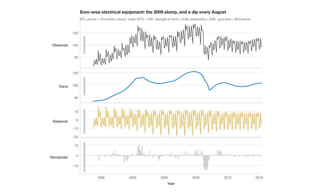
STL decomposition

A monthly industrial turnover series split into trend, seasonal and remainder components in stacked panels.

feasts::STL() + autoplot()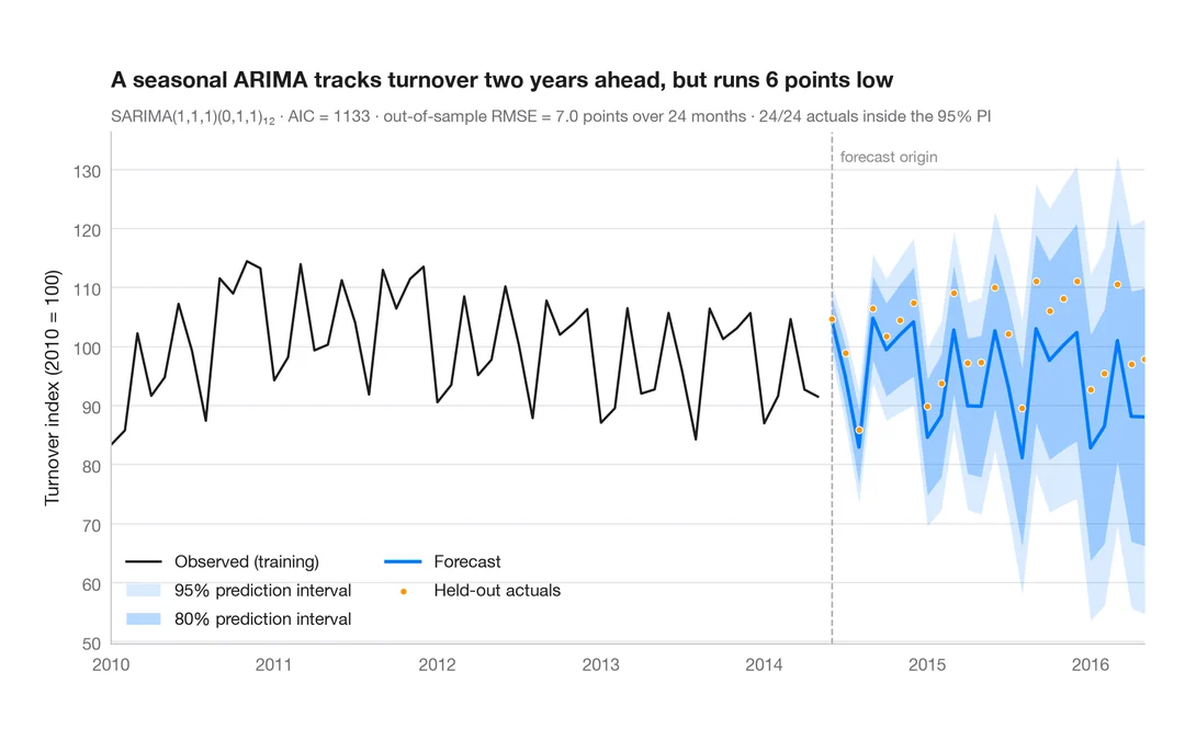

Time series

SARIMA forecast

Seasonal ARIMA forecast of industrial turnover with 80% and 95% prediction intervals against held-out data.

forecast::autoplot(forecast())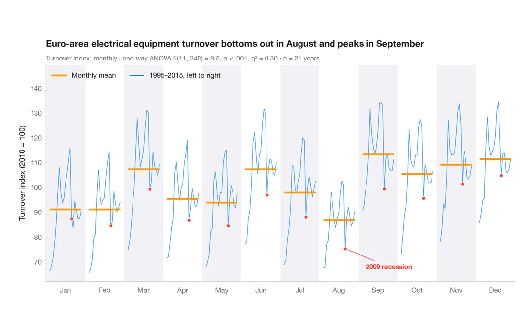

Time series

Seasonal subseries plot

Each calendar month's industrial turnover across the years, with the monthly mean as a reference.

feasts::gg_subseries()