Seasonal subseries plot

Warin, Thierry

Each calendar month's industrial turnover across the years, with the monthly mean as a reference.

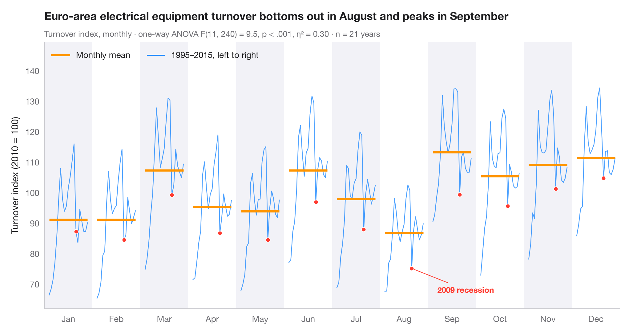
A seasonal subseries plot (or month plot) cuts a monthly series into twelve mini time series, one per calendar month, each running across all the years. The horizontal bar is that month's mean, so the shape of the season is read from bar to bar, while the line within each panel shows whether that month is drifting or swinging from year to year.

Data are Eurostat's monthly turnover index for the manufacture of electrical equipment in the euro area (2010 = 100), not seasonally adjusted, for the 21 complete years 1995–2015 (statsmodels.datasets.elec_equip, bundled with statsmodels). Turnover dips every August, when factories close for the summer, and rises at the end of each quarter. The subtitle reports a one-way ANOVA of turnover on month (scipy.stats.f_oneway) with η², the share of all variation explained by the season — modest here, because the long-run trend inside each panel accounts for much of the rest. The 2009 recession is highlighted.

seasonal-subseries.py · 53 lines

Download GitHub

import matplotlib.pyplot as plt
import numpy as np
from scipy import stats
from statsmodels.datasets import elec_equip

# Data: monthly turnover index 1995–2015, reshaped to one row per year, one column per month
turnover = elec_equip.load().data.iloc[:, 0][:"2015"]
years = turnover.index.year.unique().to_numpy()
months = turnover.index[:12].strftime("%b")
values = turnover.to_numpy().reshape(len(years), 12)

# Seasonal effect: one-way ANOVA of turnover on month, with eta squared
F, p = stats.f_oneway(*values.T)
eta2 = ((values.mean(0) - values.mean()) ** 2).sum() * len(years) / ((values - values.mean()) ** 2).sum()

fig, ax = plt.subplots(figsize=(10, 5.2))
width = 0.8
x_in = (years - years.min()) / (years.max() - years.min()) * width - width / 2
highlight = {2009: list(months)}

# One mini series per month, plus its mean
for i, m in enumerate(months):
    v = values[:, i]
    if i % 2 == 0:
        ax.axvspan(i - 0.5, i + 0.5, color="#F2F2F7", lw=0, zorder=0)
    ax.plot(i + x_in, v, color="#007AFF", lw=0.9, alpha=0.7)
    ax.hlines(v.mean(), i - width / 2, i + width / 2, color="#FF9500", lw=2.5, zorder=3)
    for yr, ms in highlight.items():
        if m in ms:
            j = np.where(years == yr)[0][0]
            ax.scatter(i + x_in[j], v[j], s=26, color="#FF3B30", edgecolor="white", lw=0.8, zorder=4)

aug09 = (7 + x_in[years == 2009][0], values[years == 2009, 7][0])
ax.annotate("2009 recession", aug09, xytext=(30, -25), textcoords="offset points",
            ha="left", va="center", fontsize=9.5,
            color="#FF3B30", fontweight="semibold",
            arrowprops=dict(arrowstyle="-", color="#FF3B30", lw=0.8))
ax.set_xticks(range(12), months)
ax.set_xlim(-0.5, 11.5)
ax.grid(axis="y")
ax.set_ylabel("Turnover index (2010 = 100)")
ax.plot([], [], color="#FF9500", lw=2.5, label="Monthly mean")
ax.plot([], [], color="#007AFF", lw=1, label=f"{years.min()}–{years.max()}, left to right")
ax.legend(loc="upper left", ncols=2)
ax.set_ylim(top=values.max() + 15)
lo_m = turnover.index[values.mean(0).argmin()].strftime("%B")   # first year runs Jan–Dec
hi_m = turnover.index[values.mean(0).argmax()].strftime("%B")
p_txt = "p < .001" if p < 0.001 else f"p = {p:.3f}"
ax.set_title(f"Euro-area electrical equipment turnover bottoms out in {lo_m} and peaks in {hi_m}", pad=26)
ax.text(0, 1.02, f"Turnover index, monthly · one-way ANOVA F(11, {values.size - 12}) = {F:.1f}, "
        f"{p_txt}, η² = {eta2:.2f} · n = {len(years)} years",
        transform=ax.transAxes, fontsize=9.5, color="#6E6E73")
plt.show()

Figures use the optional PyStatlas style: add plt.style.use("pystatlas.mplstyle") to match the look exactly.

Data source

Euro-area electrical-equipment turnover, monthly, 1995–2016. Eurostat. Euro area (18, fixed composition) total turnover index, manufacture of electrical equipment (NACE Rev. 2), working-day adjusted, not seasonally adjusted. https://ec.europa.eu/eurostat
Distributed with statsmodels (statsmodels.datasets.elec_equip); public domain.

The examples illustrate statistical methods. Their titles describe what each figure shows in these particular data — often a small, dated or partial sample — not the author's position on the substantive question. For interpretation, context and data quality, rely on the original sources cited here.

How to cite

PyStatlas is created and maintained by Thierry Warin. If it helped your work, please cite it.

Warin, T. (2026). Seasonal subseries plot. In PyStatlas: A Python Gallery of Statistical Graphics for the Social Sciences. https://warint.github.io/pystatlas/time-series/seasonal-subseries/

@misc{warin2026statlas,
  author       = {Warin, Thierry},
  title        = {PyStatlas: A Python Gallery of Statistical Graphics for the Social Sciences},
  year         = {2026},
  howpublished = {\url{https://warint.github.io/pystatlas/}},
  note         = {Source code: https://github.com/warint/pystatlas}
}

More in Time series

Time series

STL decomposition

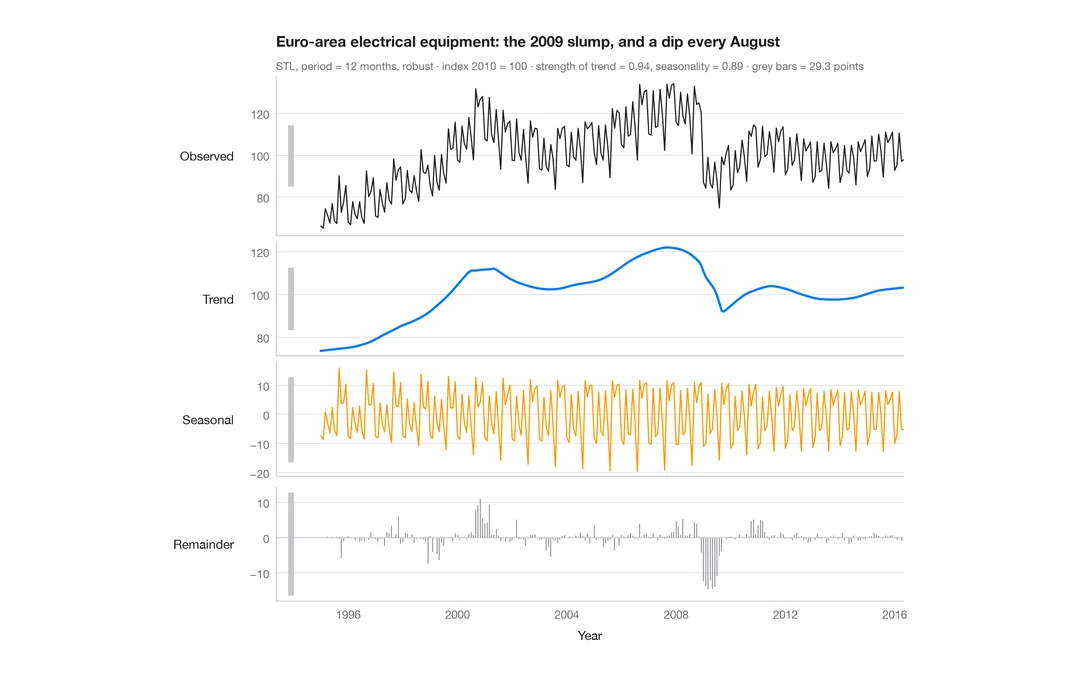
A monthly industrial turnover series split into trend, seasonal and remainder components in stacked panels.

feasts::STL() + autoplot()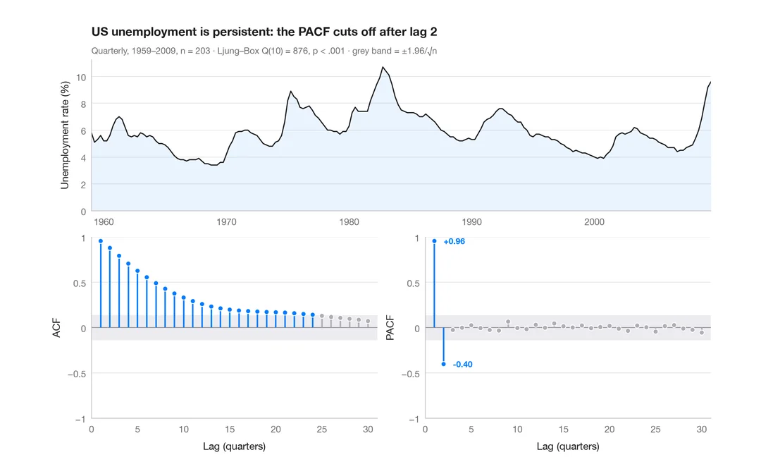

Time series

ACF and PACF

Autocorrelation and partial autocorrelation of US quarterly unemployment, as lollipops with 95% significance bands.

forecast::ggtsdisplay()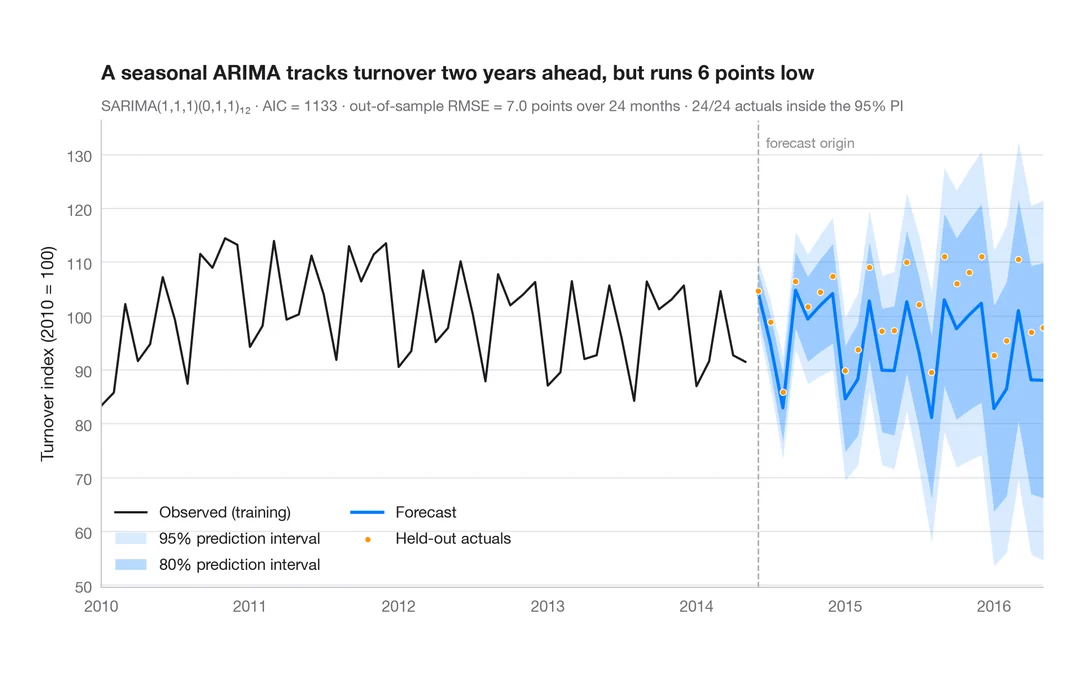

Time series

SARIMA forecast

Seasonal ARIMA forecast of industrial turnover with 80% and 95% prediction intervals against held-out data.

forecast::autoplot(forecast())