季節サブシリーズプロット
各暦月の工業売上高の年ごとの推移を、月平均を基準として示します。
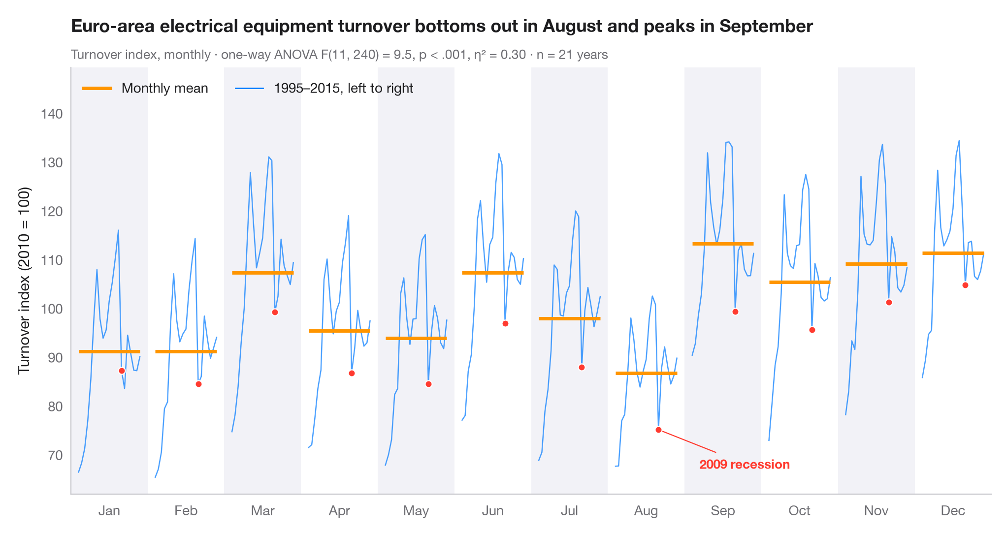
季節サブシリーズプロット(月別プロット)は、月次の時系列を暦月ごとに 12 本の小さな時系列に分け、それぞれが全年にわたって推移する様子を示します。横棒はその月の平均なので、棒から棒へと 季節のパターン を読み取ることができ、各パネル内の線はその月の値が年々ドリフトしているのか、大きく変動しているのかを示します。
データはユーロ圏の電気機器製造業の売上高に関する Eurostat の月次指数(2010 = 100、季節調整なし)で、1995–2015 年の完全な 21 年分です(statsmodels に同梱の statsmodels.datasets.elec_equip)。売上高は工場が夏季休業に入る毎年 8 月に落ち込み、各四半期末に上昇します。サブタイトルには月を要因とする売上高の一元配置分散分析(scipy.stats.f_oneway)と、総変動のうち季節で説明される割合 η² を示しています。η² がここで控えめなのは、各パネル内の長期トレンドが残りの多くを説明しているためです。2009 年の景気後退を強調表示しています。
コードおよび図中のテキストは英語です。
import matplotlib.pyplot as plt
import numpy as np
from scipy import stats
from statsmodels.datasets import elec_equip

# Data: monthly turnover index 1995–2015, reshaped to one row per year, one column per month
turnover = elec_equip.load().data.iloc[:, 0][:"2015"]
years = turnover.index.year.unique().to_numpy()
months = turnover.index[:12].strftime("%b")
values = turnover.to_numpy().reshape(len(years), 12)

# Seasonal effect: one-way ANOVA of turnover on month, with eta squared
F, p = stats.f_oneway(*values.T)
eta2 = ((values.mean(0) - values.mean()) ** 2).sum() * len(years) / ((values - values.mean()) ** 2).sum()

fig, ax = plt.subplots(figsize=(10, 5.2))
width = 0.8
x_in = (years - years.min()) / (years.max() - years.min()) * width - width / 2
highlight = {2009: list(months)}

# One mini series per month, plus its mean
for i, m in enumerate(months):
    v = values[:, i]
    if i % 2 == 0:
        ax.axvspan(i - 0.5, i + 0.5, color="#F2F2F7", lw=0, zorder=0)
    ax.plot(i + x_in, v, color="#007AFF", lw=0.9, alpha=0.7)
    ax.hlines(v.mean(), i - width / 2, i + width / 2, color="#FF9500", lw=2.5, zorder=3)
    for yr, ms in highlight.items():
        if m in ms:
            j = np.where(years == yr)[0][0]
            ax.scatter(i + x_in[j], v[j], s=26, color="#FF3B30", edgecolor="white", lw=0.8, zorder=4)

aug09 = (7 + x_in[years == 2009][0], values[years == 2009, 7][0])
ax.annotate("2009 recession", aug09, xytext=(30, -25), textcoords="offset points",
            ha="left", va="center", fontsize=9.5,
            color="#FF3B30", fontweight="semibold",
            arrowprops=dict(arrowstyle="-", color="#FF3B30", lw=0.8))
ax.set_xticks(range(12), months)
ax.set_xlim(-0.5, 11.5)
ax.grid(axis="y")
ax.set_ylabel("Turnover index (2010 = 100)")
ax.plot([], [], color="#FF9500", lw=2.5, label="Monthly mean")
ax.plot([], [], color="#007AFF", lw=1, label=f"{years.min()}–{years.max()}, left to right")
ax.legend(loc="upper left", ncols=2)
ax.set_ylim(top=values.max() + 15)
lo_m = turnover.index[values.mean(0).argmin()].strftime("%B")   # first year runs Jan–Dec
hi_m = turnover.index[values.mean(0).argmax()].strftime("%B")
p_txt = "p < .001" if p < 0.001 else f"p = {p:.3f}"
ax.set_title(f"Euro-area electrical equipment turnover bottoms out in {lo_m} and peaks in {hi_m}", pad=26)
ax.text(0, 1.02, f"Turnover index, monthly · one-way ANOVA F(11, {values.size - 12}) = {F:.1f}, "
        f"{p_txt}, η² = {eta2:.2f} · n = {len(years)} years",
        transform=ax.transAxes, fontsize=9.5, color="#6E6E73")
plt.show()
図にはオプションの PyStatlas スタイル を使用しています。同じ見た目にするには plt.style.use("pystatlas.mplstyle") を追加してください。
データの出典
- Euro-area electrical-equipment turnover, monthly, 1995–2016. Eurostat. Euro area (18, fixed composition) total turnover index, manufacture of electrical equipment (NACE Rev. 2), working-day adjusted, not seasonally adjusted. https://ec.europa.eu/eurostat
Distributed with statsmodels (statsmodels.datasets.elec_equip); public domain.
これらの例は統計手法を説明するためのものです。図のタイトルは、この特定のデータ(多くは小規模で、古く、部分的な標本)で図が示す内容を述べたものであり、実質的な問いに対する著者の立場ではありません。解釈、背景、データの質については、ここに挙げた元の出典を参照してください。
引用方法
PyStatlas は Thierry Warin が作成・運営しています。研究や業務に役立った場合は、ぜひ引用してください。
Warin, T. (2026). Seasonal subseries plot. In PyStatlas: A Python Gallery of Statistical Graphics for the Social Sciences. https://warint.github.io/pystatlas/time-series/seasonal-subseries/
@misc{warin2026statlas,
  author       = {Warin, Thierry},
  title        = {PyStatlas: A Python Gallery of Statistical Graphics for the Social Sciences},
  year         = {2026},
  howpublished = {\url{https://warint.github.io/pystatlas/}},
  note         = {Source code: https://github.com/warint/pystatlas}
}