STL decomposition — PyStatlas: A Python Gallery of Statistical Graphics for the Social Sciences

Warin, Thierry

STL 分解

月次の工業売上高の系列を、トレンド、季節成分、残差に分解して縦に並べたパネルで示します。

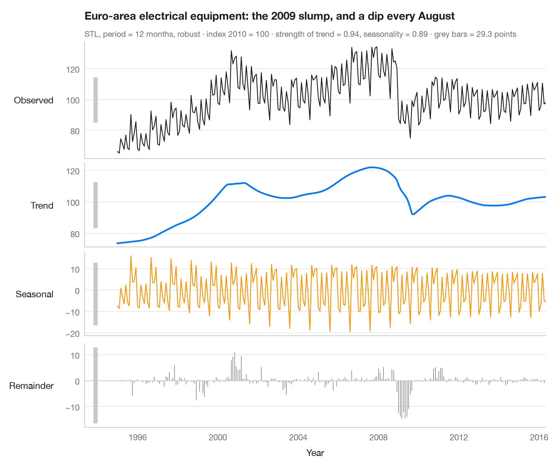
STL（Loess を用いた季節・トレンド分解）は、時系列を 観測値 = トレンド + 季節成分 + 残差 として表します。各パネルは時間軸を共有しますが縦軸のスケールはそれぞれ異なるため、各パネル左側の灰色のバー（データ単位ではすべて同じ長さ）が各成分の実際の大きさを示します。バーが短ければその成分が支配的であり、長ければその成分は小さいことを意味します。

データはユーロ圏の電気機器製造業の売上高に関する Eurostat の月次指数（2010 = 100）で、1995 年 1 月から 2016 年 5 月まで、稼働日調整済みですが季節調整は されていない 257 か月分です（statsmodels に同梱の statsmodels.datasets.elec_equip）。トレンドには 2008–09 年の工業活動の落ち込みが、季節成分には 8 月の操業停止と四半期末のピークが現れています。分解には 12 か月周期・ロバスト推定の statsmodels.tsa.seasonal.STL を用い、サブタイトルには Wang, Smith & Hyndman (2006) の定義によるトレンドと季節性の強さを示しています。

コードおよび図中のテキストは英語です。

stl-decomposition.py · 43 行

ダウンロード GitHub

import matplotlib.pyplot as plt
import numpy as np
from statsmodels.datasets import elec_equip
from statsmodels.tsa.seasonal import STL

# Data: euro-area turnover index, electrical equipment manufacturing (2010 = 100), monthly
turnover = elec_equip.load().data.iloc[:, 0]

res = STL(turnover, period=12, robust=True).fit()
parts = {"Observed": turnover, "Trend": res.trend, "Seasonal": res.seasonal, "Remainder": res.resid}
colors = ["#1D1D1F", "#007AFF", "#FF9500", "#8E8E93"]

# Strength of trend and seasonality (0 = none, 1 = all the variation)
f_trend = max(0, 1 - res.resid.var() / (res.trend + res.resid).var())
f_seas = max(0, 1 - res.resid.var() / (res.seasonal + res.resid).var())

fig, axes = plt.subplots(4, 1, figsize=(9, 7.5), sharex=True,
                         gridspec_kw=dict(height_ratios=[1.4, 1, 1, 1]))
bar = 2 * res.resid.abs().max()  # common scale bar, in index points
x0 = turnover.index[0] - np.timedelta64(400, "D")

for ax, (name, s), c in zip(axes, parts.items(), colors):
    if name == "Remainder":
        ax.vlines(s.index, 0, s, color=c, lw=0.8)
        ax.axhline(0, color="#C7C7CC", lw=0.8)
    else:
        ax.plot(s.index, s, color=c, lw=2 if name == "Trend" else 1)
    ax.set_ylabel(name, rotation=0, ha="right", va="center", labelpad=14)
    # Scale bar: same height in index points in every panel
    mid = (s.max() + s.min()) / 2
    ax.plot([x0, x0], [mid - bar / 2, mid + bar / 2], color="#C7C7CC", lw=5, solid_capstyle="butt",
            clip_on=False)

axes[-1].set_xlabel("Year")
fig.align_ylabels(axes)
axes[0].set_xlim(x0 - np.timedelta64(200, "D"), turnover.index[-1])
slump = res.trend.diff(12).idxmin().year                                  # steepest yearly fall
low = res.seasonal.groupby(res.seasonal.index.month_name()).mean().idxmin()  # weakest month
axes[0].set_title(f"Euro-area electrical equipment: the {slump} slump, and a dip every {low}", pad=26)
axes[0].text(0, 1.04, f"STL, period = 12 months, robust · index 2010 = 100 · strength of trend = "
             f"{f_trend:.2f}, seasonality = {f_seas:.2f} · grey bars = {bar:.1f} points",
             transform=axes[0].transAxes, fontsize=9.5, color="#6E6E73")
plt.show()

図にはオプションの PyStatlas スタイルを使用しています。同じ見た目にするには plt.style.use("pystatlas.mplstyle") を追加してください。

データの出典

Euro-area electrical-equipment turnover, monthly, 1995–2016. Eurostat. Euro area (18, fixed composition) total turnover index, manufacture of electrical equipment (NACE Rev. 2), working-day adjusted, not seasonally adjusted. https://ec.europa.eu/eurostat
Distributed with statsmodels (statsmodels.datasets.elec_equip); public domain.

これらの例は統計手法を説明するためのものです。図のタイトルは、この特定のデータ（多くは小規模で、古く、部分的な標本）で図が示す内容を述べたものであり、実質的な問いに対する著者の立場ではありません。解釈、背景、データの質については、ここに挙げた元の出典を参照してください。

引用方法

PyStatlas は Thierry Warin が作成・運営しています。研究や業務に役立った場合は、ぜひ引用してください。

Warin, T. (2026). STL decomposition. In PyStatlas: A Python Gallery of Statistical Graphics for the Social Sciences. https://warint.github.io/pystatlas/time-series/stl-decomposition/

@misc{warin2026statlas,
  author       = {Warin, Thierry},
  title        = {PyStatlas: A Python Gallery of Statistical Graphics for the Social Sciences},
  year         = {2026},
  howpublished = {\url{https://warint.github.io/pystatlas/}},
  note         = {Source code: https://github.com/warint/pystatlas}
}