SARIMA 予測
工業売上高の季節 ARIMA 予測を、80% と 95% の予測区間とともにホールドアウトしたデータと比較します。
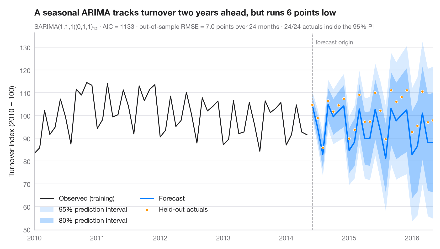
予測は不確実性とともに示してこそ誠実なものになります。濃い扇形は 80% 予測区間、薄い扇形は 95% 予測区間で、どちらも予測期間が長くなるほど広がります。最後の2年間はモデルの当てはめから 除外(ホールドアウト) しているため、点は実際に起きたことを示し、サブタイトルには標本外 RMSE と、そのうち何か月が 95% 区間に収まったかを示しています。
データはユーロ圏の電気機器製造業の売上高に関する Eurostat の月次指数(2010 = 100)で、1995 年 1 月から 2016 年 5 月まで、稼働日調整済みですが季節調整はされていません(statsmodels に同梱の statsmodels.datasets.elec_equip)。モデルは 2014 年 5 月までのデータで当てはめ、2014 年 6 月から 2016 年 5 月までを予測します。モデルは季節 ARIMA(1,1,1)(0,1,1)₁₂、いわゆる「エアライン」型の古典的な構造で、statsmodels.tsa.statespace.SARIMAX で当てはめ、区間は get_forecast().conf_int() によるものです。ホールドアウトしたすべての月が 95% 区間に収まっていますが、予測は平均して実際の値を下回っています。
コードおよび図中のテキストは英語です。
import matplotlib.pyplot as plt
import numpy as np
from statsmodels.datasets import elec_equip
from statsmodels.tsa.statespace.sarimax import SARIMAX

# Data: euro-area turnover index, electrical equipment (2010 = 100); hold out the last 2 years
turnover = elec_equip.load().data.iloc[:, 0].asfreq("MS")
h = 24
train, test = turnover[:-h], turnover[-h:]

# Fit a seasonal ARIMA and forecast the held-out horizon
fit = SARIMAX(train, order=(1, 1, 1), seasonal_order=(0, 1, 1, 12)).fit(disp=False)
fc = fit.get_forecast(h)
mean, ci95, ci80 = fc.predicted_mean, fc.conf_int(alpha=0.05), fc.conf_int(alpha=0.20)

rmse = np.sqrt(((test - mean) ** 2).mean())
bias = (test - mean).mean()                       # > 0: actuals above the forecast
covered = ((test >= ci95.iloc[:, 0]) & (test <= ci95.iloc[:, 1])).sum()

fig, ax = plt.subplots(figsize=(9, 5))
hist = train["2010":]
ax.plot(hist.index, hist, color="#1D1D1F", lw=1.4, label="Observed (training)")
ax.fill_between(mean.index, ci95.iloc[:, 0], ci95.iloc[:, 1], color="#007AFF", alpha=0.15, lw=0,
                label="95% prediction interval")
ax.fill_between(mean.index, ci80.iloc[:, 0], ci80.iloc[:, 1], color="#007AFF", alpha=0.28, lw=0,
                label="80% prediction interval")
ax.plot(mean.index, mean, color="#007AFF", lw=2, label="Forecast")
ax.scatter(test.index, test, s=16, color="#FF9500", edgecolor="white", lw=0.6, zorder=4,
           label="Held-out actuals")

# Mark the forecast origin
ax.axvline(test.index[0], color="#AEAEB2", lw=1, ls="--")
ax.text(test.index[0], 0.97, "  forecast origin", transform=ax.get_xaxis_transform(),
        fontsize=9, color="#8E8E93", va="top")

ax.set(ylabel="Turnover index (2010 = 100)", xlim=(hist.index[0], test.index[-1]))
ax.legend(loc="lower left", ncols=2)
ax.set_title(f"A seasonal ARIMA tracks turnover two years ahead, but runs {abs(bias):.0f} points "
             f"{'low' if bias > 0 else 'high'}", pad=26)
ax.text(0, 1.02, f"SARIMA(1,1,1)(0,1,1)₁₂ · AIC = {fit.aic:.0f} · out-of-sample RMSE = {rmse:.1f} points "
        f"over {h} months · {covered}/{h} actuals inside the 95% PI",
        transform=ax.transAxes, fontsize=9.5, color="#6E6E73")
plt.show()
図にはオプションの PyStatlas スタイル を使用しています。同じ見た目にするには plt.style.use("pystatlas.mplstyle") を追加してください。
データの出典
- Euro-area electrical-equipment turnover, monthly, 1995–2016. Eurostat. Euro area (18, fixed composition) total turnover index, manufacture of electrical equipment (NACE Rev. 2), working-day adjusted, not seasonally adjusted. https://ec.europa.eu/eurostat
Distributed with statsmodels (statsmodels.datasets.elec_equip); public domain.
これらの例は統計手法を説明するためのものです。図のタイトルは、この特定のデータ(多くは小規模で、古く、部分的な標本)で図が示す内容を述べたものであり、実質的な問いに対する著者の立場ではありません。解釈、背景、データの質については、ここに挙げた元の出典を参照してください。
引用方法
PyStatlas は Thierry Warin が作成・運営しています。研究や業務に役立った場合は、ぜひ引用してください。
Warin, T. (2026). SARIMA forecast. In PyStatlas: A Python Gallery of Statistical Graphics for the Social Sciences. https://warint.github.io/pystatlas/time-series/arima-forecast/
@misc{warin2026statlas,
  author       = {Warin, Thierry},
  title        = {PyStatlas: A Python Gallery of Statistical Graphics for the Social Sciences},
  year         = {2026},
  howpublished = {\url{https://warint.github.io/pystatlas/}},
  note         = {Source code: https://github.com/warint/pystatlas}
}