SARIMA 预测
工业营业额的季节性 ARIMA 预测,附 80% 和 95% 预测区间,并与留出数据对照。
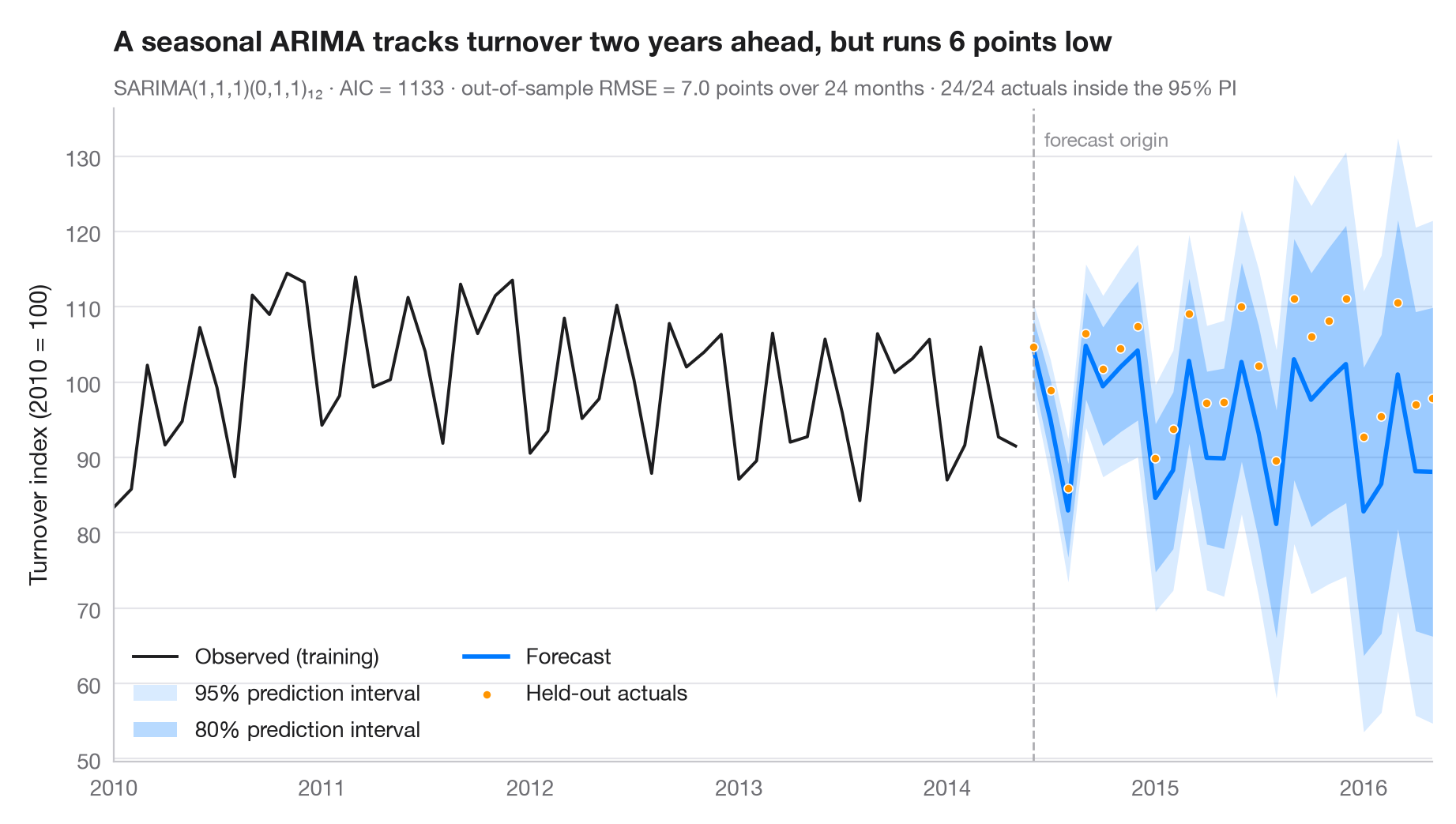
只有附带不确定性,预测才是诚实的。深色扇形为 80% 预测区间,浅色扇形为 95% 区间;两者都随预测期延长而变宽。最后两年数据在拟合时被留出,因此圆点显示的是实际发生的情况,副标题报告样本外 RMSE,以及这些月份中有多少落在 95% 区间之内。
数据为 Eurostat 发布的欧元区电气设备制造业月度营业额指数(2010 = 100),1995 年 1 月至 2016 年 5 月,经工作日调整但未经季节调整(statsmodels.datasets.elec_equip,随 statsmodels 提供)。模型用截至 2014 年 5 月的数据拟合,预测 2014 年 6 月至 2016 年 5 月。模型为季节性 ARIMA(1,1,1)(0,1,1)₁₂——经典的“航空”结构——用 statsmodels.tsa.statespace.SARIMAX 拟合;区间来自 get_forecast().conf_int()。所有留出月份都落在 95% 区间之内,但预测平均低于实际值。
代码及图中文字均为英文。
import matplotlib.pyplot as plt
import numpy as np
from statsmodels.datasets import elec_equip
from statsmodels.tsa.statespace.sarimax import SARIMAX

# Data: euro-area turnover index, electrical equipment (2010 = 100); hold out the last 2 years
turnover = elec_equip.load().data.iloc[:, 0].asfreq("MS")
h = 24
train, test = turnover[:-h], turnover[-h:]

# Fit a seasonal ARIMA and forecast the held-out horizon
fit = SARIMAX(train, order=(1, 1, 1), seasonal_order=(0, 1, 1, 12)).fit(disp=False)
fc = fit.get_forecast(h)
mean, ci95, ci80 = fc.predicted_mean, fc.conf_int(alpha=0.05), fc.conf_int(alpha=0.20)

rmse = np.sqrt(((test - mean) ** 2).mean())
bias = (test - mean).mean()                       # > 0: actuals above the forecast
covered = ((test >= ci95.iloc[:, 0]) & (test <= ci95.iloc[:, 1])).sum()

fig, ax = plt.subplots(figsize=(9, 5))
hist = train["2010":]
ax.plot(hist.index, hist, color="#1D1D1F", lw=1.4, label="Observed (training)")
ax.fill_between(mean.index, ci95.iloc[:, 0], ci95.iloc[:, 1], color="#007AFF", alpha=0.15, lw=0,
                label="95% prediction interval")
ax.fill_between(mean.index, ci80.iloc[:, 0], ci80.iloc[:, 1], color="#007AFF", alpha=0.28, lw=0,
                label="80% prediction interval")
ax.plot(mean.index, mean, color="#007AFF", lw=2, label="Forecast")
ax.scatter(test.index, test, s=16, color="#FF9500", edgecolor="white", lw=0.6, zorder=4,
           label="Held-out actuals")

# Mark the forecast origin
ax.axvline(test.index[0], color="#AEAEB2", lw=1, ls="--")
ax.text(test.index[0], 0.97, "  forecast origin", transform=ax.get_xaxis_transform(),
        fontsize=9, color="#8E8E93", va="top")

ax.set(ylabel="Turnover index (2010 = 100)", xlim=(hist.index[0], test.index[-1]))
ax.legend(loc="lower left", ncols=2)
ax.set_title(f"A seasonal ARIMA tracks turnover two years ahead, but runs {abs(bias):.0f} points "
             f"{'low' if bias > 0 else 'high'}", pad=26)
ax.text(0, 1.02, f"SARIMA(1,1,1)(0,1,1)₁₂ · AIC = {fit.aic:.0f} · out-of-sample RMSE = {rmse:.1f} points "
        f"over {h} months · {covered}/{h} actuals inside the 95% PI",
        transform=ax.transAxes, fontsize=9.5, color="#6E6E73")
plt.show()
图表使用了可选的 PyStatlas 样式:添加 plt.style.use("pystatlas.mplstyle") 即可完全还原其外观。
数据来源
- Euro-area electrical-equipment turnover, monthly, 1995–2016. Eurostat. Euro area (18, fixed composition) total turnover index, manufacture of electrical equipment (NACE Rev. 2), working-day adjusted, not seasonally adjusted. https://ec.europa.eu/eurostat
Distributed with statsmodels (statsmodels.datasets.elec_equip); public domain.
这些示例用于说明统计方法。图表标题描述的是该图在这些特定数据中呈现的内容——这些数据往往样本较小、年代较早或并不完整——而不是作者对实质问题的立场。关于解释、背景和数据质量,请以此处引用的原始来源为准。
如何引用
PyStatlas 由 Thierry Warin 创建并维护。如果它对你的工作有所帮助,敬请引用。
Warin, T. (2026). SARIMA forecast. In PyStatlas: A Python Gallery of Statistical Graphics for the Social Sciences. https://warint.github.io/pystatlas/time-series/arima-forecast/
@misc{warin2026statlas,
  author       = {Warin, Thierry},
  title        = {PyStatlas: A Python Gallery of Statistical Graphics for the Social Sciences},
  year         = {2026},
  howpublished = {\url{https://warint.github.io/pystatlas/}},
  note         = {Source code: https://github.com/warint/pystatlas}
}