ACF 与 PACF
美国季度失业率的自相关与偏自相关,以棒棒糖图展示并附 95% 显著性带。
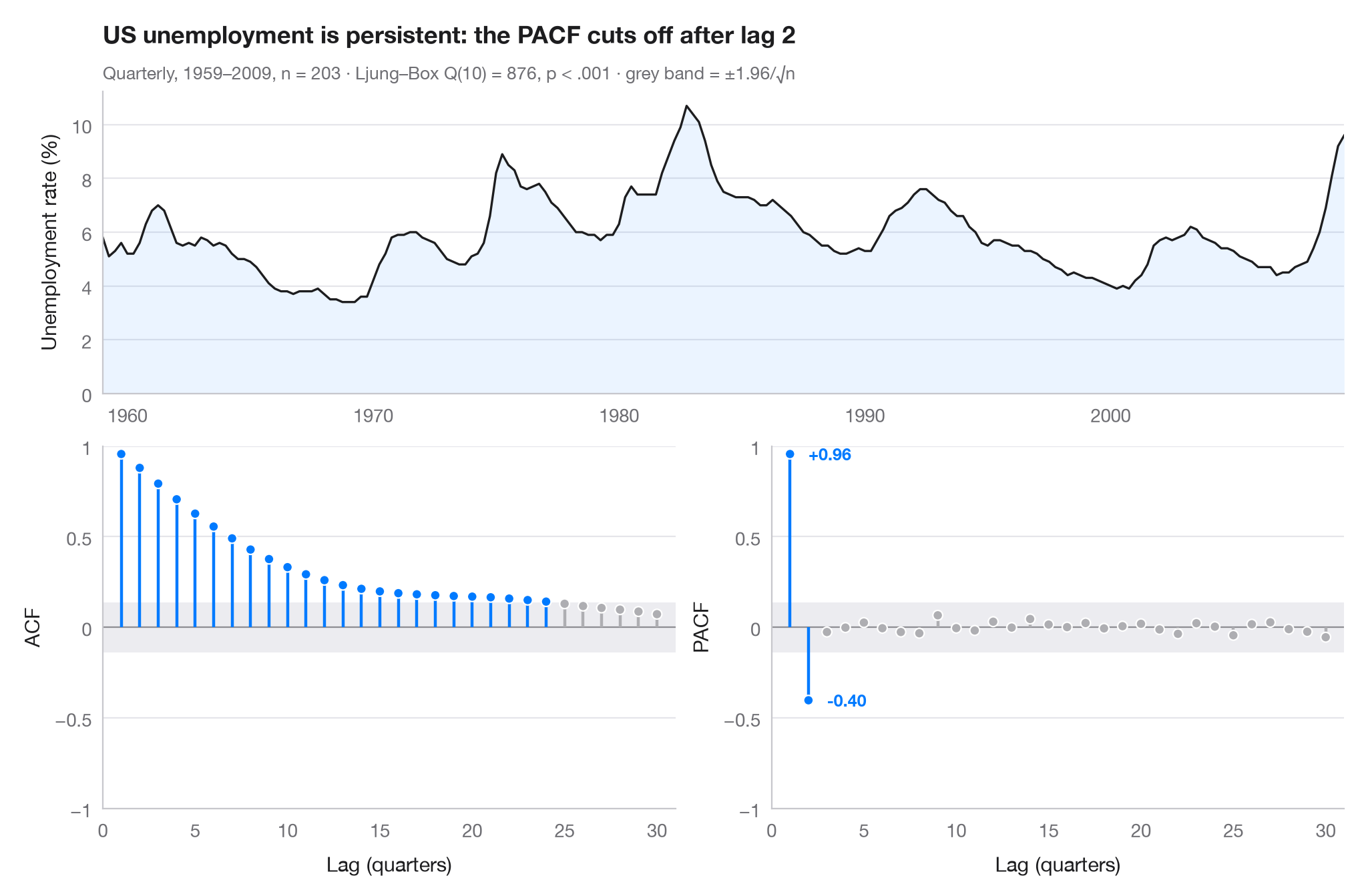
自相关函数(ACF)衡量序列与其自身 k 步之前的值的相关程度;偏自相关函数(PACF)则在剔除中间较短滞后的影响后做同样的衡量。超出灰色带(±1.96/√n)的竖线大于白噪声所能产生的水平。两个面板结合起来可提示合适的模型:这里 ACF 在数年间缓慢衰减——今天失业率高,明年失业率也高——而 PACF 在两个滞后之后截尾,这正是 AR(2) 过程的特征。
数据为美国平民失业率,1959 年第 1 季度至 2009 年第 3 季度的季度数据(203 个季度),取自 statsmodels 自带的宏观经济数据集(sm.datasets.macrodata,列 unemp)。相关系数来自 statsmodels.tsa.stattools.acf 和 pacf,副标题报告无自相关的 Ljung–Box 检验。
代码及图中文字均为英文。
import matplotlib.pyplot as plt
import numpy as np
import statsmodels.api as sm
from statsmodels.stats.diagnostic import acorr_ljungbox
from statsmodels.tsa.stattools import acf, pacf

# Data: US unemployment rate, quarterly
df = sm.datasets.macrodata.load_pandas().data
y = df.set_index(df.year + (df.quarter - 1) / 4)["unemp"]
n, nlags = len(y), 30
band = 1.96 / np.sqrt(n)
lb = acorr_ljungbox(y, lags=[10]).iloc[0]

fig = plt.figure(figsize=(10, 6.5))
gs = fig.add_gridspec(2, 2, height_ratios=[1, 1.2])
ax_ts = fig.add_subplot(gs[0, :])
axes = [fig.add_subplot(gs[1, 0]), fig.add_subplot(gs[1, 1])]

# Top: the series itself
ax_ts.plot(y.index, y, color="#1D1D1F", lw=1.2)
ax_ts.fill_between(y.index, y, color="#007AFF", alpha=0.08, lw=0)
ax_ts.set(ylabel="Unemployment rate (%)", xlim=(y.index[0], y.index[-1]), ylim=(0, None))

# Bottom: ACF and PACF as lollipops with the white-noise band
values = [acf(y, nlags=nlags)[1:], pacf(y, nlags=nlags, method="ywm")[1:]]
for ax, v, name in zip(axes, values, ["ACF", "PACF"]):
    lags = np.arange(1, nlags + 1)
    sig = np.abs(v) > band
    colors = np.where(sig, "#007AFF", "#AEAEB2")
    ax.axhspan(-band, band, color="#E5E5EA", alpha=0.7, lw=0)
    ax.axhline(0, color="#8E8E93", lw=0.8)
    ax.vlines(lags, 0, v, color=colors, lw=1.6)
    ax.scatter(lags, v, s=28, color=colors, edgecolor="white", lw=0.8, zorder=3)
    ax.set(xlabel="Lag (quarters)", ylabel=name, ylim=(-1, 1), xlim=(0, nlags + 1))
    ax.set_xticks(range(0, nlags + 1, 5))
    ax.set_yticks([-1, -0.5, 0, 0.5, 1], ["−1", "−0.5", "0", "0.5", "1"])
last = np.flatnonzero(np.abs(values[1]) > band)[-1] + 1     # last significant PACF lag
for lag in (1, last):
    axes[1].annotate(f"{values[1][lag - 1]:+.2f}", (lag, values[1][lag - 1]),
                     xytext=(10, 0), textcoords="offset points", va="center",
                     fontsize=9, color="#007AFF", fontweight="semibold")

ax_ts.set_title(f"US unemployment is persistent: the PACF cuts off after lag {last}", pad=26)
p_txt = "p < .001" if lb.lb_pvalue < 0.001 else f"p = {lb.lb_pvalue:.3f}"
ax_ts.text(0, 1.04, f"Quarterly, 1959–2009, n = {n} · Ljung–Box Q(10) = {lb.lb_stat:.0f}, "
           f"{p_txt} · grey band = ±1.96/√n", transform=ax_ts.transAxes, fontsize=9.5, color="#6E6E73")
plt.show()
图表使用了可选的 PyStatlas 样式:添加 plt.style.use("pystatlas.mplstyle") 即可完全还原其外观。
数据来源
- US quarterly macroeconomic series, 1959–2009. Federal Reserve Bank of St. Louis. FRED, Federal Reserve Economic Data; U.S. Bureau of Labor Statistics (unemployment rate). Accessed December 15, 2009. https://fred.stlouisfed.org/
Compiled by Skipper Seabold for statsmodels (sm.datasets.macrodata); public domain.
这些示例用于说明统计方法。图表标题描述的是该图在这些特定数据中呈现的内容——这些数据往往样本较小、年代较早或并不完整——而不是作者对实质问题的立场。关于解释、背景和数据质量,请以此处引用的原始来源为准。
如何引用
PyStatlas 由 Thierry Warin 创建并维护。如果它对你的工作有所帮助,敬请引用。
Warin, T. (2026). ACF and PACF. In PyStatlas: A Python Gallery of Statistical Graphics for the Social Sciences. https://warint.github.io/pystatlas/time-series/acf-pacf/
@misc{warin2026statlas,
  author       = {Warin, Thierry},
  title        = {PyStatlas: A Python Gallery of Statistical Graphics for the Social Sciences},
  year         = {2026},
  howpublished = {\url{https://warint.github.io/pystatlas/}},
  note         = {Source code: https://github.com/warint/pystatlas}
}