ACF と PACF
米国の四半期失業率の自己相関と偏自己相関を、95% 有意帯付きのロリポップで示します。
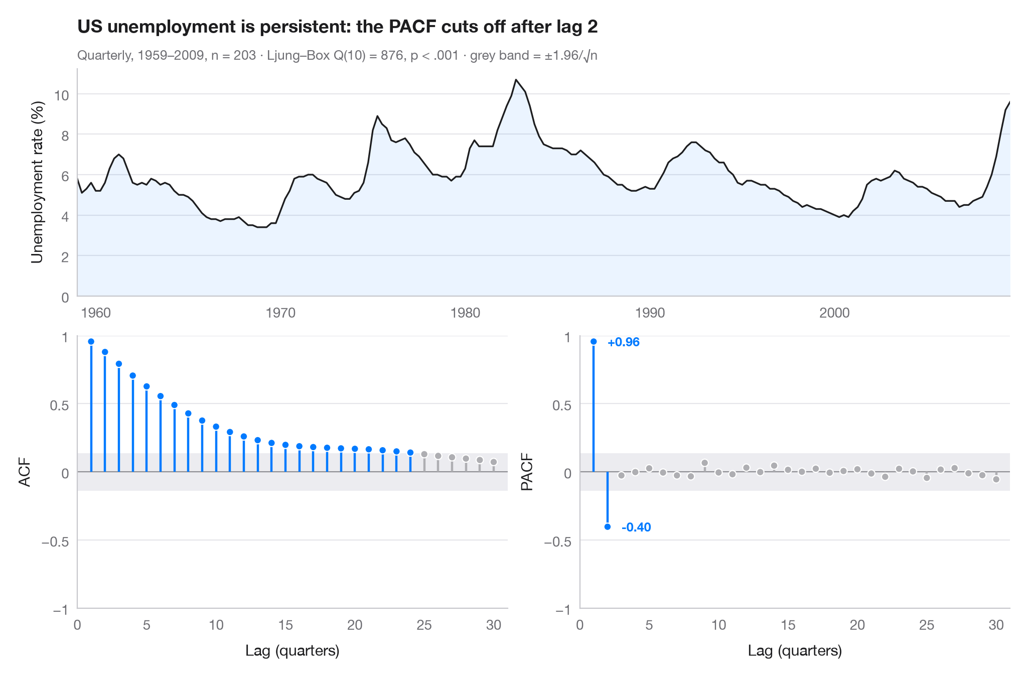
自己相関関数(ACF)は、時系列が k 期前の自分自身とどの程度強く相関しているかを測ります。偏自己相関(PACF)は、その間にある短いラグの影響を取り除いたうえで同じことを行います。灰色の帯(±1.96/√n)からはみ出す棒は、ホワイトノイズから生じる値より大きいものです。2つのパネルを合わせて見ると、モデルの見当が付きます。ここでは ACF が数年にわたってゆっくり減衰する(今日の失業率が高ければ来年も高い)一方、PACF は 2 ラグ で切断されており、これは AR(2) 過程の特徴です。
データは米国の民間失業率で、1959 年第 1 四半期から 2009 年第 3 四半期までの四半期データ(203 四半期)です。statsmodels に同梱のマクロ経済データセット(sm.datasets.macrodata、列 unemp)から取っています。相関は statsmodels.tsa.stattools.acf と pacf によるもので、サブタイトルには自己相関なしを帰無仮説とするリュン・ボックス検定を示しています。
コードおよび図中のテキストは英語です。
import matplotlib.pyplot as plt
import numpy as np
import statsmodels.api as sm
from statsmodels.stats.diagnostic import acorr_ljungbox
from statsmodels.tsa.stattools import acf, pacf

# Data: US unemployment rate, quarterly
df = sm.datasets.macrodata.load_pandas().data
y = df.set_index(df.year + (df.quarter - 1) / 4)["unemp"]
n, nlags = len(y), 30
band = 1.96 / np.sqrt(n)
lb = acorr_ljungbox(y, lags=[10]).iloc[0]

fig = plt.figure(figsize=(10, 6.5))
gs = fig.add_gridspec(2, 2, height_ratios=[1, 1.2])
ax_ts = fig.add_subplot(gs[0, :])
axes = [fig.add_subplot(gs[1, 0]), fig.add_subplot(gs[1, 1])]

# Top: the series itself
ax_ts.plot(y.index, y, color="#1D1D1F", lw=1.2)
ax_ts.fill_between(y.index, y, color="#007AFF", alpha=0.08, lw=0)
ax_ts.set(ylabel="Unemployment rate (%)", xlim=(y.index[0], y.index[-1]), ylim=(0, None))

# Bottom: ACF and PACF as lollipops with the white-noise band
values = [acf(y, nlags=nlags)[1:], pacf(y, nlags=nlags, method="ywm")[1:]]
for ax, v, name in zip(axes, values, ["ACF", "PACF"]):
    lags = np.arange(1, nlags + 1)
    sig = np.abs(v) > band
    colors = np.where(sig, "#007AFF", "#AEAEB2")
    ax.axhspan(-band, band, color="#E5E5EA", alpha=0.7, lw=0)
    ax.axhline(0, color="#8E8E93", lw=0.8)
    ax.vlines(lags, 0, v, color=colors, lw=1.6)
    ax.scatter(lags, v, s=28, color=colors, edgecolor="white", lw=0.8, zorder=3)
    ax.set(xlabel="Lag (quarters)", ylabel=name, ylim=(-1, 1), xlim=(0, nlags + 1))
    ax.set_xticks(range(0, nlags + 1, 5))
    ax.set_yticks([-1, -0.5, 0, 0.5, 1], ["−1", "−0.5", "0", "0.5", "1"])
last = np.flatnonzero(np.abs(values[1]) > band)[-1] + 1     # last significant PACF lag
for lag in (1, last):
    axes[1].annotate(f"{values[1][lag - 1]:+.2f}", (lag, values[1][lag - 1]),
                     xytext=(10, 0), textcoords="offset points", va="center",
                     fontsize=9, color="#007AFF", fontweight="semibold")

ax_ts.set_title(f"US unemployment is persistent: the PACF cuts off after lag {last}", pad=26)
p_txt = "p < .001" if lb.lb_pvalue < 0.001 else f"p = {lb.lb_pvalue:.3f}"
ax_ts.text(0, 1.04, f"Quarterly, 1959–2009, n = {n} · Ljung–Box Q(10) = {lb.lb_stat:.0f}, "
           f"{p_txt} · grey band = ±1.96/√n", transform=ax_ts.transAxes, fontsize=9.5, color="#6E6E73")
plt.show()
図にはオプションの PyStatlas スタイル を使用しています。同じ見た目にするには plt.style.use("pystatlas.mplstyle") を追加してください。
データの出典
- US quarterly macroeconomic series, 1959–2009. Federal Reserve Bank of St. Louis. FRED, Federal Reserve Economic Data; U.S. Bureau of Labor Statistics (unemployment rate). Accessed December 15, 2009. https://fred.stlouisfed.org/
Compiled by Skipper Seabold for statsmodels (sm.datasets.macrodata); public domain.
これらの例は統計手法を説明するためのものです。図のタイトルは、この特定のデータ(多くは小規模で、古く、部分的な標本)で図が示す内容を述べたものであり、実質的な問いに対する著者の立場ではありません。解釈、背景、データの質については、ここに挙げた元の出典を参照してください。
引用方法
PyStatlas は Thierry Warin が作成・運営しています。研究や業務に役立った場合は、ぜひ引用してください。
Warin, T. (2026). ACF and PACF. In PyStatlas: A Python Gallery of Statistical Graphics for the Social Sciences. https://warint.github.io/pystatlas/time-series/acf-pacf/
@misc{warin2026statlas,
  author       = {Warin, Thierry},
  title        = {PyStatlas: A Python Gallery of Statistical Graphics for the Social Sciences},
  year         = {2026},
  howpublished = {\url{https://warint.github.io/pystatlas/}},
  note         = {Source code: https://github.com/warint/pystatlas}
}