STL 分解
将月度工业营业额序列分解为趋势、季节和残余成分,并以堆叠面板展示。
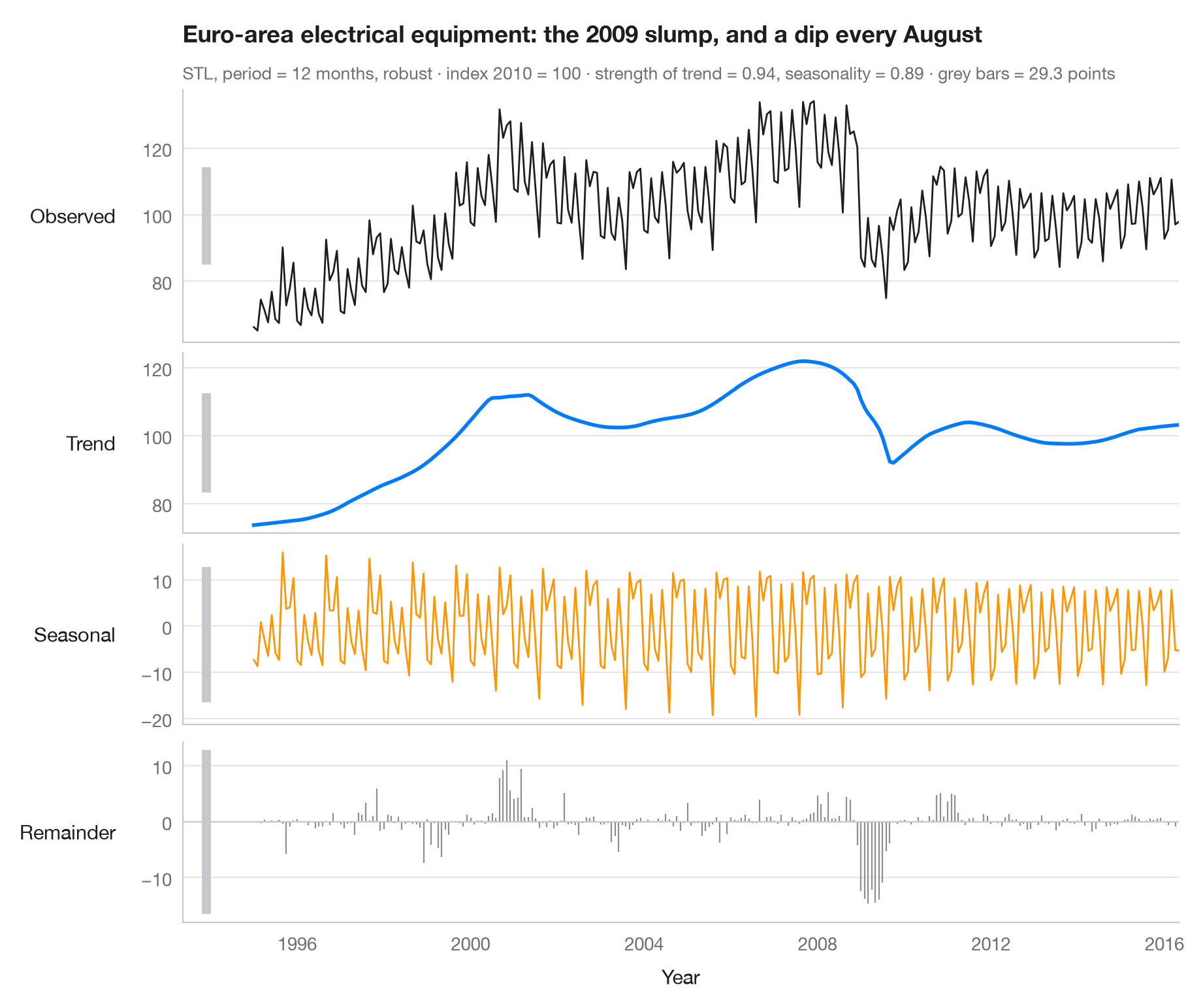
STL(基于 Loess 的季节–趋势分解)将序列写成观测值 = 趋势 + 季节 + 残余。各面板共用时间轴,但纵轴刻度各自独立,因此每个面板左侧的灰色竖条——在数据单位上长度完全相同——显示了每个成分的真实大小:竖条短,说明该成分占主导;竖条长,说明该成分较小。
数据为 Eurostat 发布的欧元区电气设备制造业月度营业额指数(2010 = 100),1995 年 1 月至 2016 年 5 月,经工作日调整但未经季节调整——共 257 个月,随 statsmodels 提供(statsmodels.datasets.elec_equip)。趋势显示了 2008–09 年工业活动的崩塌;季节成分显示了 8 月停工和季度末的高峰。分解使用 statsmodels.tsa.seasonal.STL,周期为 12 个月并采用稳健拟合;副标题给出按 Wang、Smith 和 Hyndman(2006)定义的趋势强度和季节强度。
代码及图中文字均为英文。
import matplotlib.pyplot as plt
import numpy as np
from statsmodels.datasets import elec_equip
from statsmodels.tsa.seasonal import STL

# Data: euro-area turnover index, electrical equipment manufacturing (2010 = 100), monthly
turnover = elec_equip.load().data.iloc[:, 0]

res = STL(turnover, period=12, robust=True).fit()
parts = {"Observed": turnover, "Trend": res.trend, "Seasonal": res.seasonal, "Remainder": res.resid}
colors = ["#1D1D1F", "#007AFF", "#FF9500", "#8E8E93"]

# Strength of trend and seasonality (0 = none, 1 = all the variation)
f_trend = max(0, 1 - res.resid.var() / (res.trend + res.resid).var())
f_seas = max(0, 1 - res.resid.var() / (res.seasonal + res.resid).var())

fig, axes = plt.subplots(4, 1, figsize=(9, 7.5), sharex=True,
                         gridspec_kw=dict(height_ratios=[1.4, 1, 1, 1]))
bar = 2 * res.resid.abs().max()  # common scale bar, in index points
x0 = turnover.index[0] - np.timedelta64(400, "D")

for ax, (name, s), c in zip(axes, parts.items(), colors):
    if name == "Remainder":
        ax.vlines(s.index, 0, s, color=c, lw=0.8)
        ax.axhline(0, color="#C7C7CC", lw=0.8)
    else:
        ax.plot(s.index, s, color=c, lw=2 if name == "Trend" else 1)
    ax.set_ylabel(name, rotation=0, ha="right", va="center", labelpad=14)
    # Scale bar: same height in index points in every panel
    mid = (s.max() + s.min()) / 2
    ax.plot([x0, x0], [mid - bar / 2, mid + bar / 2], color="#C7C7CC", lw=5, solid_capstyle="butt",
            clip_on=False)

axes[-1].set_xlabel("Year")
fig.align_ylabels(axes)
axes[0].set_xlim(x0 - np.timedelta64(200, "D"), turnover.index[-1])
slump = res.trend.diff(12).idxmin().year                                  # steepest yearly fall
low = res.seasonal.groupby(res.seasonal.index.month_name()).mean().idxmin()  # weakest month
axes[0].set_title(f"Euro-area electrical equipment: the {slump} slump, and a dip every {low}", pad=26)
axes[0].text(0, 1.04, f"STL, period = 12 months, robust · index 2010 = 100 · strength of trend = "
             f"{f_trend:.2f}, seasonality = {f_seas:.2f} · grey bars = {bar:.1f} points",
             transform=axes[0].transAxes, fontsize=9.5, color="#6E6E73")
plt.show()
图表使用了可选的 PyStatlas 样式:添加 plt.style.use("pystatlas.mplstyle") 即可完全还原其外观。
数据来源
- Euro-area electrical-equipment turnover, monthly, 1995–2016. Eurostat. Euro area (18, fixed composition) total turnover index, manufacture of electrical equipment (NACE Rev. 2), working-day adjusted, not seasonally adjusted. https://ec.europa.eu/eurostat
Distributed with statsmodels (statsmodels.datasets.elec_equip); public domain.
这些示例用于说明统计方法。图表标题描述的是该图在这些特定数据中呈现的内容——这些数据往往样本较小、年代较早或并不完整——而不是作者对实质问题的立场。关于解释、背景和数据质量,请以此处引用的原始来源为准。
如何引用
PyStatlas 由 Thierry Warin 创建并维护。如果它对你的工作有所帮助,敬请引用。
Warin, T. (2026). STL decomposition. In PyStatlas: A Python Gallery of Statistical Graphics for the Social Sciences. https://warint.github.io/pystatlas/time-series/stl-decomposition/
@misc{warin2026statlas,
  author       = {Warin, Thierry},
  title        = {PyStatlas: A Python Gallery of Statistical Graphics for the Social Sciences},
  year         = {2026},
  howpublished = {\url{https://warint.github.io/pystatlas/}},
  note         = {Source code: https://github.com/warint/pystatlas}
}