SARIMA forecast

Warin, Thierry

Seasonal ARIMA forecast of industrial turnover with 80% and 95% prediction intervals against held-out data.

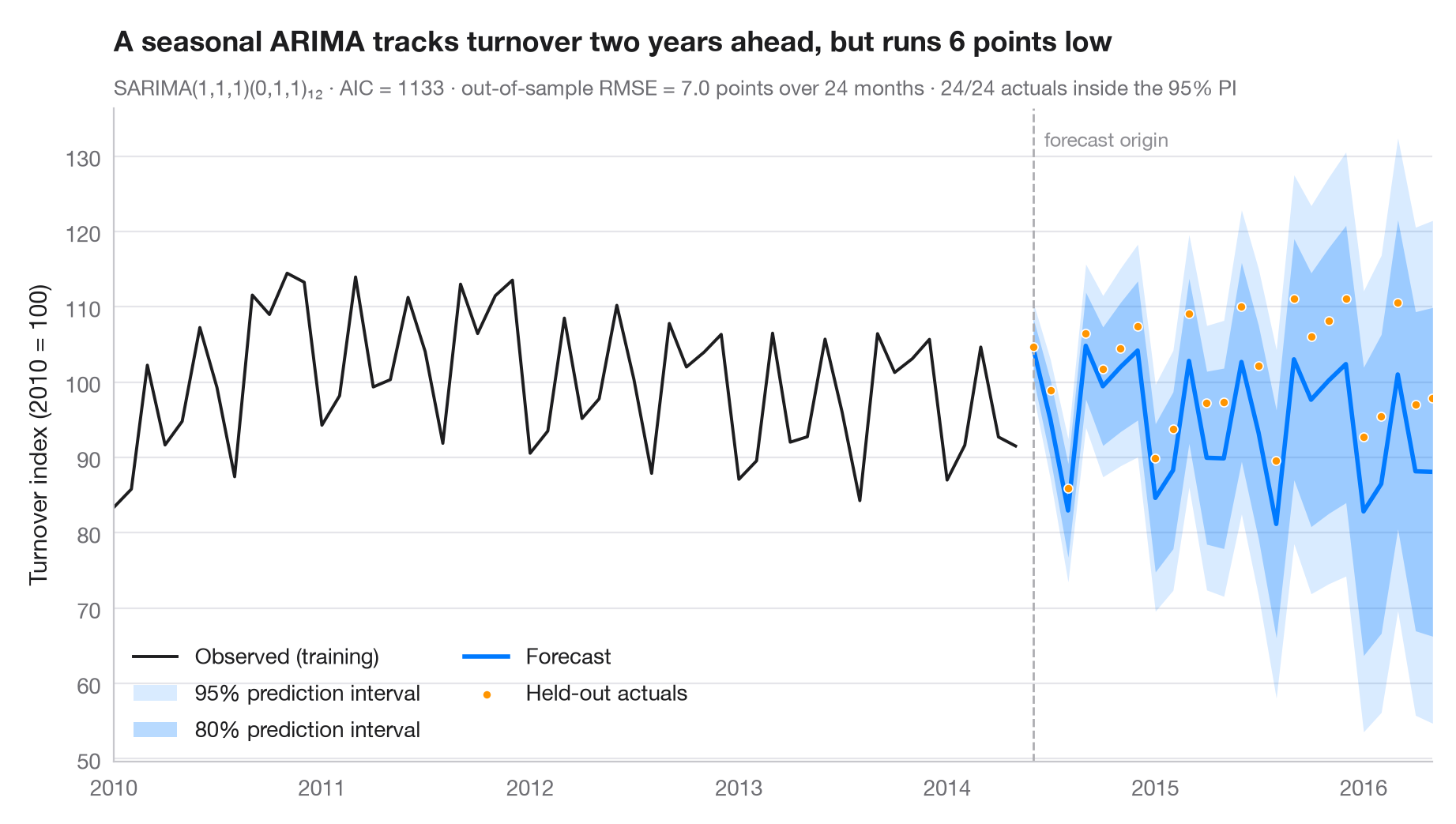
A forecast is only honest with its uncertainty. The dark fan is the 80% prediction interval, the light fan the 95% interval; both widen as the horizon grows. The last two years were held out from the fit, so the dots show what actually happened and the subtitle reports the out-of-sample RMSE and how many of those months fell inside the 95% interval.

Data are Eurostat's monthly turnover index for the manufacture of electrical equipment in the euro area (2010 = 100), January 1995 to May 2016, working-day adjusted but not seasonally adjusted (statsmodels.datasets.elec_equip, bundled with statsmodels). The model is fitted on data up to May 2014 and forecasts June 2014 – May 2016. It is a seasonal ARIMA(1,1,1)(0,1,1)₁₂ — the classic "airline" structure — fitted with statsmodels.tsa.statespace.SARIMAX; intervals come from get_forecast().conf_int(). Every held-out month falls inside the 95% interval, but the forecast sits below the actual values on average.

arima-forecast.py · 43 lines

Download GitHub

import matplotlib.pyplot as plt
import numpy as np
from statsmodels.datasets import elec_equip
from statsmodels.tsa.statespace.sarimax import SARIMAX

# Data: euro-area turnover index, electrical equipment (2010 = 100); hold out the last 2 years
turnover = elec_equip.load().data.iloc[:, 0].asfreq("MS")
h = 24
train, test = turnover[:-h], turnover[-h:]

# Fit a seasonal ARIMA and forecast the held-out horizon
fit = SARIMAX(train, order=(1, 1, 1), seasonal_order=(0, 1, 1, 12)).fit(disp=False)
fc = fit.get_forecast(h)
mean, ci95, ci80 = fc.predicted_mean, fc.conf_int(alpha=0.05), fc.conf_int(alpha=0.20)

rmse = np.sqrt(((test - mean) ** 2).mean())
bias = (test - mean).mean()                       # > 0: actuals above the forecast
covered = ((test >= ci95.iloc[:, 0]) & (test <= ci95.iloc[:, 1])).sum()

fig, ax = plt.subplots(figsize=(9, 5))
hist = train["2010":]
ax.plot(hist.index, hist, color="#1D1D1F", lw=1.4, label="Observed (training)")
ax.fill_between(mean.index, ci95.iloc[:, 0], ci95.iloc[:, 1], color="#007AFF", alpha=0.15, lw=0,
                label="95% prediction interval")
ax.fill_between(mean.index, ci80.iloc[:, 0], ci80.iloc[:, 1], color="#007AFF", alpha=0.28, lw=0,
                label="80% prediction interval")
ax.plot(mean.index, mean, color="#007AFF", lw=2, label="Forecast")
ax.scatter(test.index, test, s=16, color="#FF9500", edgecolor="white", lw=0.6, zorder=4,
           label="Held-out actuals")

# Mark the forecast origin
ax.axvline(test.index[0], color="#AEAEB2", lw=1, ls="--")
ax.text(test.index[0], 0.97, "  forecast origin", transform=ax.get_xaxis_transform(),
        fontsize=9, color="#8E8E93", va="top")

ax.set(ylabel="Turnover index (2010 = 100)", xlim=(hist.index[0], test.index[-1]))
ax.legend(loc="lower left", ncols=2)
ax.set_title(f"A seasonal ARIMA tracks turnover two years ahead, but runs {abs(bias):.0f} points "
             f"{'low' if bias > 0 else 'high'}", pad=26)
ax.text(0, 1.02, f"SARIMA(1,1,1)(0,1,1)₁₂ · AIC = {fit.aic:.0f} · out-of-sample RMSE = {rmse:.1f} points "
        f"over {h} months · {covered}/{h} actuals inside the 95% PI",
        transform=ax.transAxes, fontsize=9.5, color="#6E6E73")
plt.show()

Figures use the optional PyStatlas style: add plt.style.use("pystatlas.mplstyle") to match the look exactly.

Data source

Euro-area electrical-equipment turnover, monthly, 1995–2016. Eurostat. Euro area (18, fixed composition) total turnover index, manufacture of electrical equipment (NACE Rev. 2), working-day adjusted, not seasonally adjusted. https://ec.europa.eu/eurostat
Distributed with statsmodels (statsmodels.datasets.elec_equip); public domain.

The examples illustrate statistical methods. Their titles describe what each figure shows in these particular data — often a small, dated or partial sample — not the author's position on the substantive question. For interpretation, context and data quality, rely on the original sources cited here.

How to cite

PyStatlas is created and maintained by Thierry Warin. If it helped your work, please cite it.

Warin, T. (2026). SARIMA forecast. In PyStatlas: A Python Gallery of Statistical Graphics for the Social Sciences. https://warint.github.io/pystatlas/time-series/arima-forecast/

@misc{warin2026statlas,
  author       = {Warin, Thierry},
  title        = {PyStatlas: A Python Gallery of Statistical Graphics for the Social Sciences},
  year         = {2026},
  howpublished = {\url{https://warint.github.io/pystatlas/}},
  note         = {Source code: https://github.com/warint/pystatlas}
}

More in Time series

Time series

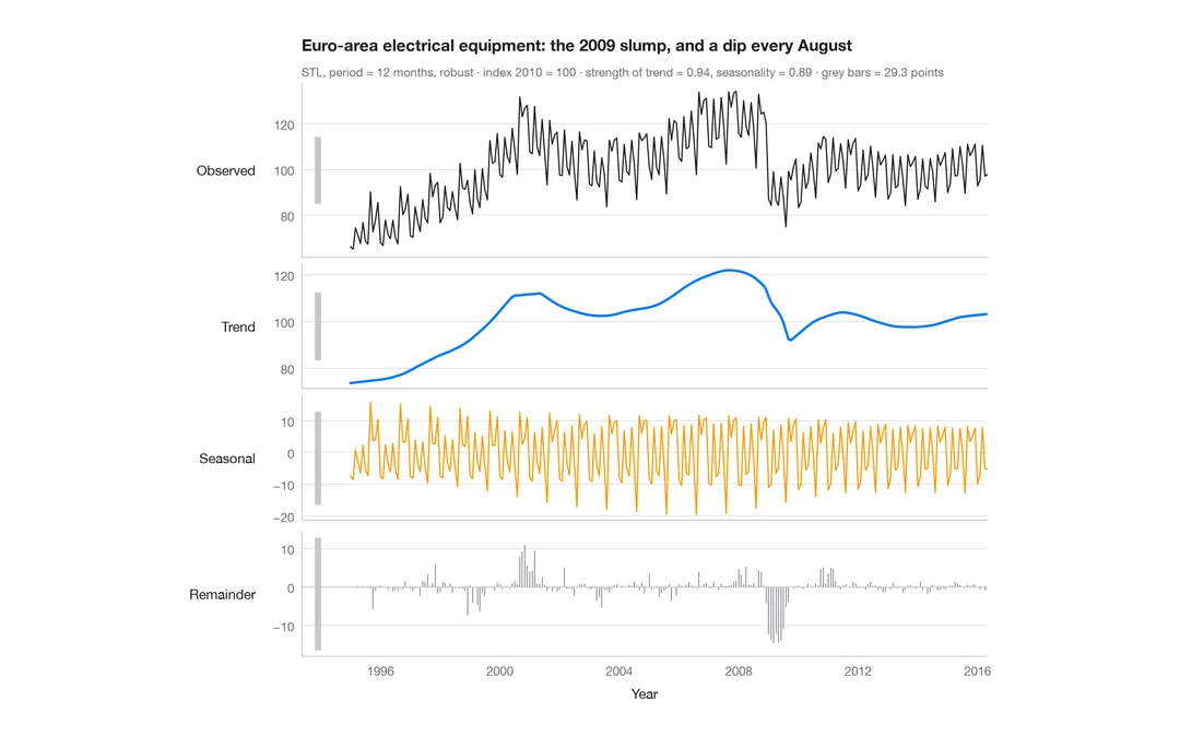
STL decomposition

A monthly industrial turnover series split into trend, seasonal and remainder components in stacked panels.

feasts::STL() + autoplot()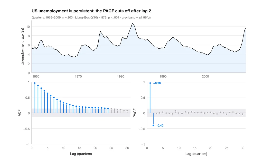

Time series

ACF and PACF

Autocorrelation and partial autocorrelation of US quarterly unemployment, as lollipops with 95% significance bands.

forecast::ggtsdisplay()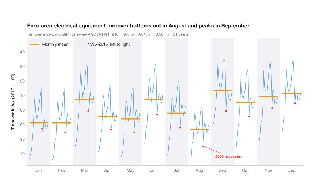

Time series

Seasonal subseries plot

Each calendar month's industrial turnover across the years, with the monthly mean as a reference.

feasts::gg_subseries()