ROC curves
Three classifiers compared by ROC curve, AUC with bootstrap 95% CI and Youden point.
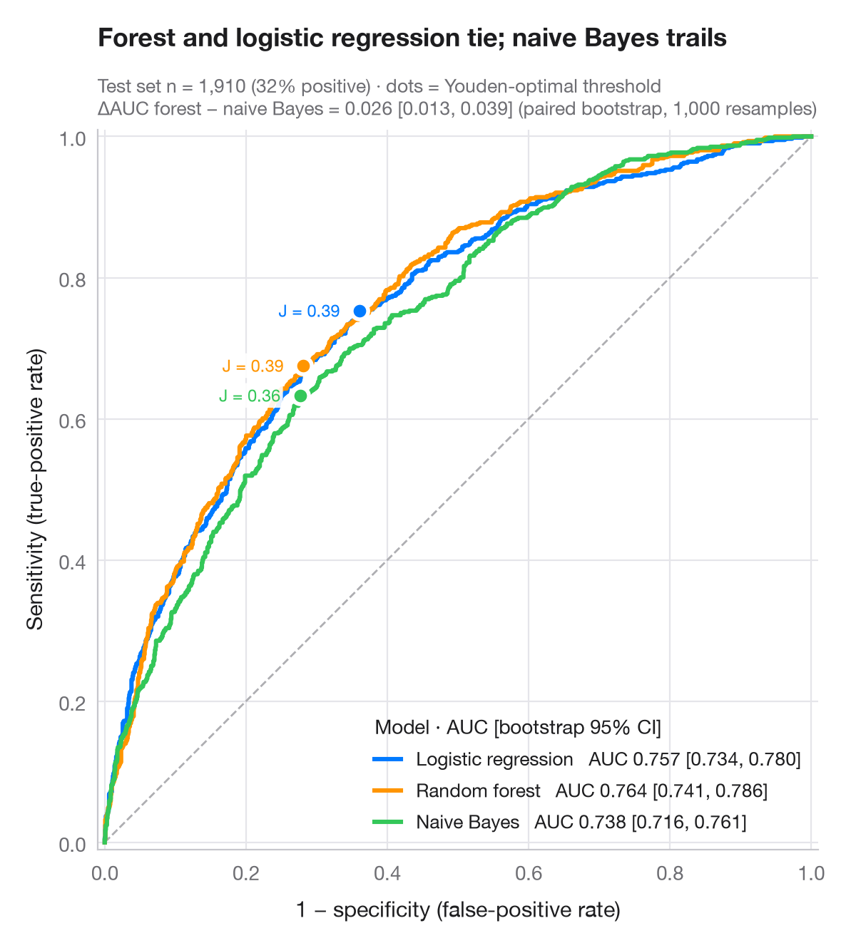
A ROC curve traces sensitivity against 1 − specificity as the decision threshold sweeps from strict to lenient. The diagonal is a coin flip; the closer a curve hugs the top-left corner, the better. The AUC is the probability that a random positive case scores higher than a random negative one; its 95% interval comes from 1,000 bootstrap resamples of the test set, and a paired bootstrap compares the best and weakest model. The dot on each curve is the threshold that maximises Youden's J = sensitivity + specificity − 1.
Data are the 6,366 respondents of Fair's affairs survey (sm.datasets.fair),
split 70/30 into training and test sets. A logistic regression, a random forest
and a naive Bayes model from scikit-learn predict whether a respondent
reported an affair; curves and AUCs come from roc_curve() and roc_auc_score().
import matplotlib.pyplot as plt
import numpy as np
import statsmodels.api as sm
from sklearn.ensemble import RandomForestClassifier
from sklearn.linear_model import LogisticRegression
from sklearn.metrics import roc_auc_score, roc_curve
from sklearn.model_selection import train_test_split
from sklearn.naive_bayes import GaussianNB

# Data: predict any affair from the survey answers
df = sm.datasets.fair.load_pandas().data
X, y = df.drop(columns="affairs").to_numpy(), (df.affairs > 0).astype(int).to_numpy()
X_tr, X_te, y_tr, y_te = train_test_split(X, y, test_size=0.3, stratify=y, random_state=1)

models = {"Logistic regression": LogisticRegression(max_iter=1000),
          "Random forest": RandomForestClassifier(300, min_samples_leaf=20, random_state=1),
          "Naive Bayes": GaussianNB()}
palette = ["#007AFF", "#FF9500", "#34C759"]
rng = np.random.default_rng(42)
boot = [rng.integers(0, len(y_te), len(y_te)) for _ in range(1000)]

fig, ax = plt.subplots(figsize=(7, 6.4))
ax.plot([0, 1], [0, 1], color="#AEAEB2", lw=1, ls="--")
scores = {}
for (name, clf), c in zip(models.items(), palette):
    score = scores[name] = clf.fit(X_tr, y_tr).predict_proba(X_te)[:, 1]
    fpr, tpr, thr = roc_curve(y_te, score)
    auc = roc_auc_score(y_te, score)
    lo, hi = np.percentile([roc_auc_score(y_te[b], score[b]) for b in boot], [2.5, 97.5])
    ax.plot(fpr, tpr, color=c, lw=2.2, label=f"{name}   AUC {auc:.3f} [{lo:.3f}, {hi:.3f}]")
    # Youden's J: threshold that maximises TPR − FPR
    j = np.argmax(tpr - fpr)
    ax.scatter(fpr[j], tpr[j], s=70, color=c, edgecolor="white", lw=2, zorder=5)
    ax.annotate(f"J = {tpr[j] - fpr[j]:.2f}", (fpr[j], tpr[j]), xytext=(-10, 0),
                textcoords="offset points", fontsize=8.5, color=c, ha="right", va="center",
                bbox=dict(boxstyle="round,pad=0.15", fc="white", ec="none", alpha=0.9))

# Paired bootstrap: is the best model really better than the weakest?
a, b = scores["Random forest"], scores["Naive Bayes"]
diff = [roc_auc_score(y_te[i], a[i]) - roc_auc_score(y_te[i], b[i]) for i in boot]
d_lo, d_hi = np.percentile(diff, [2.5, 97.5])

ax.set_xlim(-0.01, 1.01); ax.set_ylim(-0.01, 1.01); ax.set_aspect("equal")
ax.grid(axis="x")
ax.set_xlabel("1 − specificity (false-positive rate)")
ax.set_ylabel("Sensitivity (true-positive rate)")
ax.legend(loc="lower right", title="Model · AUC [bootstrap 95% CI]", alignment="left",
          handlelength=1.4, fontsize=9.5)
ax.set_title("Forest and logistic regression tie; naive Bayes trails", pad=42)
ax.text(0, 1.02, f"Test set n = {len(y_te):,} ({y_te.mean():.0%} positive) · dots = Youden-optimal threshold\n"
        f"ΔAUC forest − naive Bayes = {roc_auc_score(y_te, a) - roc_auc_score(y_te, b):.3f} "
        f"[{d_lo:.3f}, {d_hi:.3f}] (paired bootstrap, 1,000 resamples)",
        transform=ax.transAxes, fontsize=9.5, color="#6E6E73")
plt.show()
Figures use the optional PyStatlas style: add plt.style.use("pystatlas.mplstyle") to match the look exactly.
Data source
- Redbook survey of married women, 1974 (Fair's affairs data). Fair, R. C. (1978). A theory of extramarital affairs. Journal of Political Economy, 86(1), 45–61. https://doi.org/10.1086/260646
Data from the 1974 Redbook magazine survey; distributed with statsmodels (sm.datasets.fair) with the author's permission.
The examples illustrate statistical methods. Their titles describe what each figure shows in these particular data — often a small, dated or partial sample — not the author's position on the substantive question. For interpretation, context and data quality, rely on the original sources cited here.
How to cite
PyStatlas is created and maintained by Thierry Warin. If it helped your work, please cite it.
Warin, T. (2026). ROC curves. In PyStatlas: A Python Gallery of Statistical Graphics for the Social Sciences. https://warint.github.io/pystatlas/model-diagnostics/roc-curve/
@misc{warin2026statlas,
  author       = {Warin, Thierry},
  title        = {PyStatlas: A Python Gallery of Statistical Graphics for the Social Sciences},
  year         = {2026},
  howpublished = {\url{https://warint.github.io/pystatlas/}},
  note         = {Source code: https://github.com/warint/pystatlas}
}More in Model diagnostics
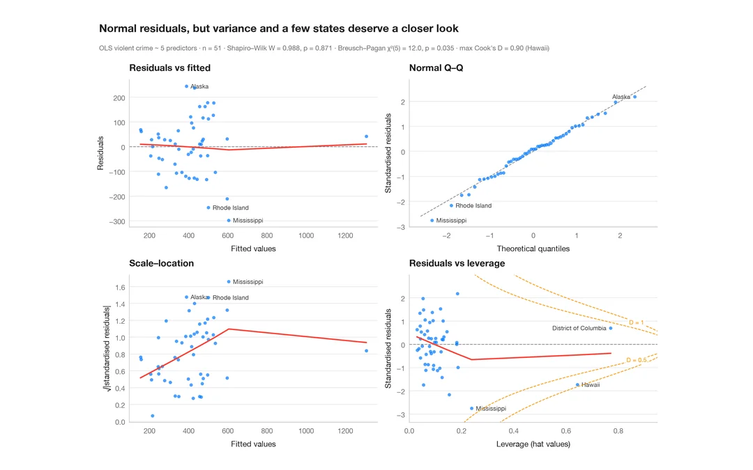
Residual diagnostics
The classic 2 × 2 panel for a linear model — linearity, normality, variance, leverage.
plot(lm) / performance::check_model()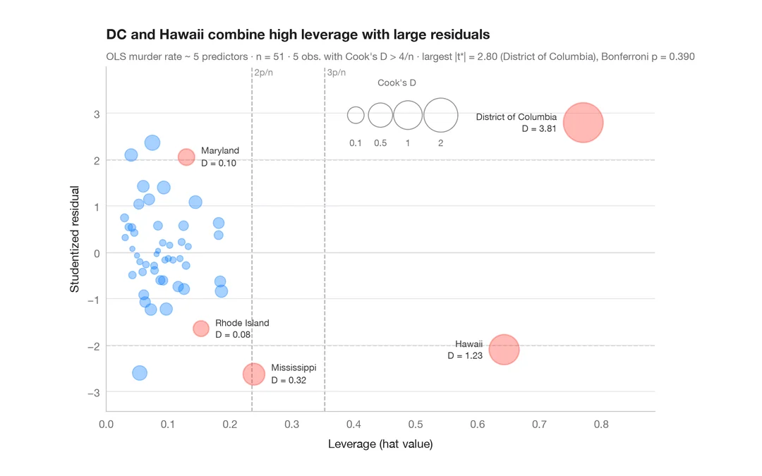
Influence plot
Studentized residuals vs leverage, with bubbles sized by Cook's distance.
car::influencePlot()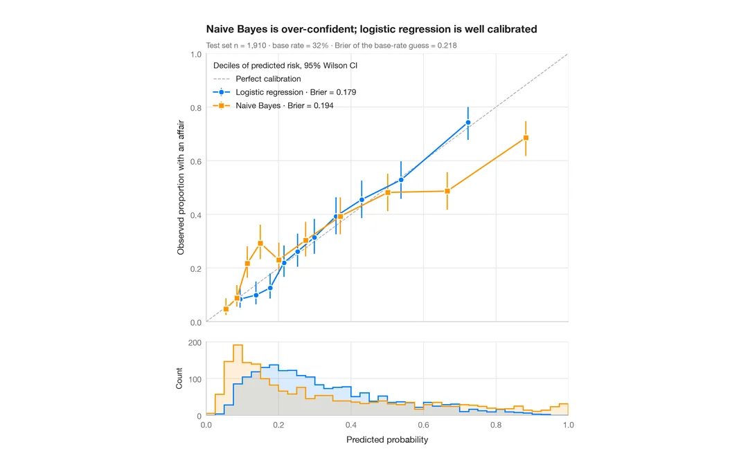
Calibration plot
Predicted vs observed risk per decile, with Wilson CIs, prediction histograms and Brier score.
rms::calibrate() / probably::cal_plot_breaks()