Residual diagnostics
The classic 2 × 2 panel for a linear model — linearity, normality, variance, leverage.
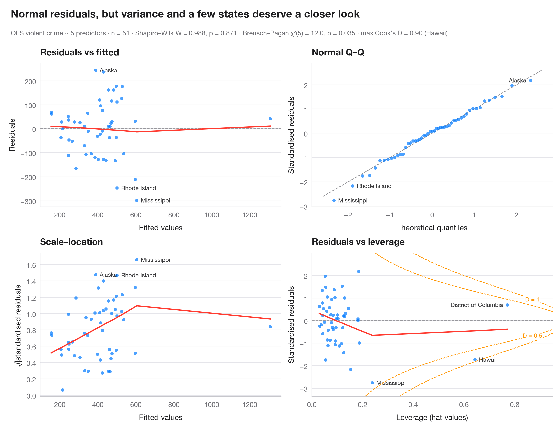
Four views of the residuals answer four questions. Residuals vs fitted: is the relationship linear (flat LOWESS curve)? Normal Q–Q: are residuals roughly normal (points on the line)? Scale–location: is the spread constant (flat curve)? Residuals vs leverage: does any observation pull the fit, i.e. sits beyond the dashed Cook's distance contours? The three most extreme observations are labelled in each panel, and formal tests sit in the subtitle.
The model is the violent-crime regression on the 50 US states + DC from
sm.datasets.statecrime. Everything comes from get_influence() in
statsmodels, plus lowess() for the smoothers, het_breuschpagan() and
scipy.stats.shapiro().
import matplotlib.pyplot as plt
import numpy as np
import statsmodels.api as sm
import statsmodels.formula.api as smf
from scipy import stats
from statsmodels.nonparametric.smoothers_lowess import lowess
from statsmodels.stats.diagnostic import het_breuschpagan

df = sm.datasets.statecrime.load_pandas().data
model = smf.ols("violent ~ poverty + single + urban + hs_grad + white", data=df).fit()
infl = model.get_influence()
fitted, resid = model.fittedvalues, model.resid
std_r, lev, cook = infl.resid_studentized_internal, infl.hat_matrix_diag, infl.cooks_distance[0]
p = model.df_model + 1
top = np.argsort(-np.abs(std_r))[:3]                # 3 largest standardised residuals

fig, axes = plt.subplots(2, 2, figsize=(11, 7.6))
kw = dict(s=22, color="#007AFF", alpha=0.7, lw=0, zorder=2)
smooth = dict(color="#FF3B30", lw=1.8)

def label(ax, x, y, idx):
    lo, hi = ax.get_xlim()
    for i in idx:                                   # text on the side with more room
        right = (x[i] - lo) / (hi - lo) < 0.75
        ax.annotate(df.index[i], (x[i], y[i]), xytext=(6 if right else -6, 0),
                    textcoords="offset points", ha="left" if right else "right",
                    va="center", fontsize=8.5, color="#3A3A3C", zorder=1,
                    bbox=dict(boxstyle="round,pad=0.15", fc="white", ec="none", alpha=0.85))


# 1. Residuals vs fitted
ax = axes[0, 0]
ax.axhline(0, color="#8E8E93", lw=1, ls="--")
ax.scatter(fitted, resid, **kw)
ax.plot(*lowess(resid, fitted, frac=1, it=0).T, **smooth)
label(ax, fitted.values, resid.values, top)
ax.set(title="Residuals vs fitted", xlabel="Fitted values", ylabel="Residuals")

# 2. Normal Q-Q of standardised residuals
ax = axes[0, 1]
order = np.argsort(std_r)
theo = stats.norm.ppf((np.arange(1, len(std_r) + 1) - 0.5) / len(std_r))
ax.plot([-2.6, 2.6], [-2.6, 2.6], color="#8E8E93", lw=1, ls="--")
ax.scatter(theo, std_r[order], **kw)
rank = {i: k for k, i in enumerate(order)}
label(ax, {i: theo[rank[i]] for i in top}, std_r, top)
ax.set(title="Normal Q–Q", xlabel="Theoretical quantiles", ylabel="Standardised residuals")

# 3. Scale-location
ax = axes[1, 0]
root = np.sqrt(np.abs(std_r))
ax.scatter(fitted, root, **kw)
ax.plot(*lowess(root, fitted, frac=1, it=0).T, **smooth)
label(ax, fitted.values, np.abs(root), top)
ax.set(title="Scale–location", xlabel="Fitted values", ylabel="√|standardised residuals|")

# 4. Residuals vs leverage with Cook's distance contours
ax = axes[1, 1]
ax.axhline(0, color="#8E8E93", lw=1, ls="--")
ax.scatter(lev, std_r, **kw)
ax.plot(*lowess(std_r, lev, frac=1, it=0).T, **smooth)
ylim = (std_r.min() - 0.6, std_r.max() + 0.8)
h = np.linspace(0.01, 0.95, 300)
for D in (0.5, 1):
    r = np.sqrt(D * p * (1 - h) / h)
    ax.plot(h, r, color="#FF9500", lw=1, ls="--"); ax.plot(h, -r, color="#FF9500", lw=1, ls="--")
    sign = 1 if D == 1 else -1                       # label D = 1 above, D = 0.5 below
    ax.text(0.87, sign * np.sqrt(D * p * 0.13 / 0.87), f"D = {D}", color="#FF9500", fontsize=8.5,
            ha="center", va="center", bbox=dict(boxstyle="round,pad=0.15", fc="white", ec="none"))
ax.set_ylim(*ylim); ax.set_xlim(0, 0.95)
label(ax, lev, std_r, np.argsort(-cook)[:3])
ax.set(title="Residuals vs leverage", xlabel="Leverage (hat values)", ylabel="Standardised residuals")
for a in axes.flat:
    a.title.set_fontsize(12)

bp = het_breuschpagan(resid, model.model.exog)
sw = stats.shapiro(resid)
fig.text(0.01, 1.065, "Normal residuals, but variance and a few states deserve a closer look",
         fontsize=15, fontweight="semibold", va="bottom")
fig.text(0.01, 1.02, f"OLS violent crime ~ 5 predictors · n = {int(model.nobs)} · Shapiro–Wilk "
         f"W = {sw.statistic:.3f}, p = {sw.pvalue:.3f} · Breusch–Pagan χ²({p - 1:.0f}) = "
         f"{bp[0]:.1f}, p = {bp[1]:.3f} · max Cook's D = {cook.max():.2f} ({df.index[cook.argmax()]})",
         fontsize=9.5, color="#6E6E73", va="bottom")
plt.show()
Figures use the optional PyStatlas style: add plt.style.use("pystatlas.mplstyle") to match the look exactly.
Data source
- US state crime and social indicators, 2009. U.S. Census Bureau. Statistical Abstract of the United States, state tables for 2009 (crime rates from the FBI Uniform Crime Reporting program). https://www.statsmodels.org/stable/datasets/generated/statecrime.html
Compiled for statsmodels (sm.datasets.statecrime); public domain. See the statsmodels page for each variable's table and footnotes.
The examples illustrate statistical methods. Their titles describe what each figure shows in these particular data — often a small, dated or partial sample — not the author's position on the substantive question. For interpretation, context and data quality, rely on the original sources cited here.
How to cite
PyStatlas is created and maintained by Thierry Warin. If it helped your work, please cite it.
Warin, T. (2026). Residual diagnostics. In PyStatlas: A Python Gallery of Statistical Graphics for the Social Sciences. https://warint.github.io/pystatlas/model-diagnostics/residual-diagnostics/
@misc{warin2026statlas,
  author       = {Warin, Thierry},
  title        = {PyStatlas: A Python Gallery of Statistical Graphics for the Social Sciences},
  year         = {2026},
  howpublished = {\url{https://warint.github.io/pystatlas/}},
  note         = {Source code: https://github.com/warint/pystatlas}
}More in Model diagnostics
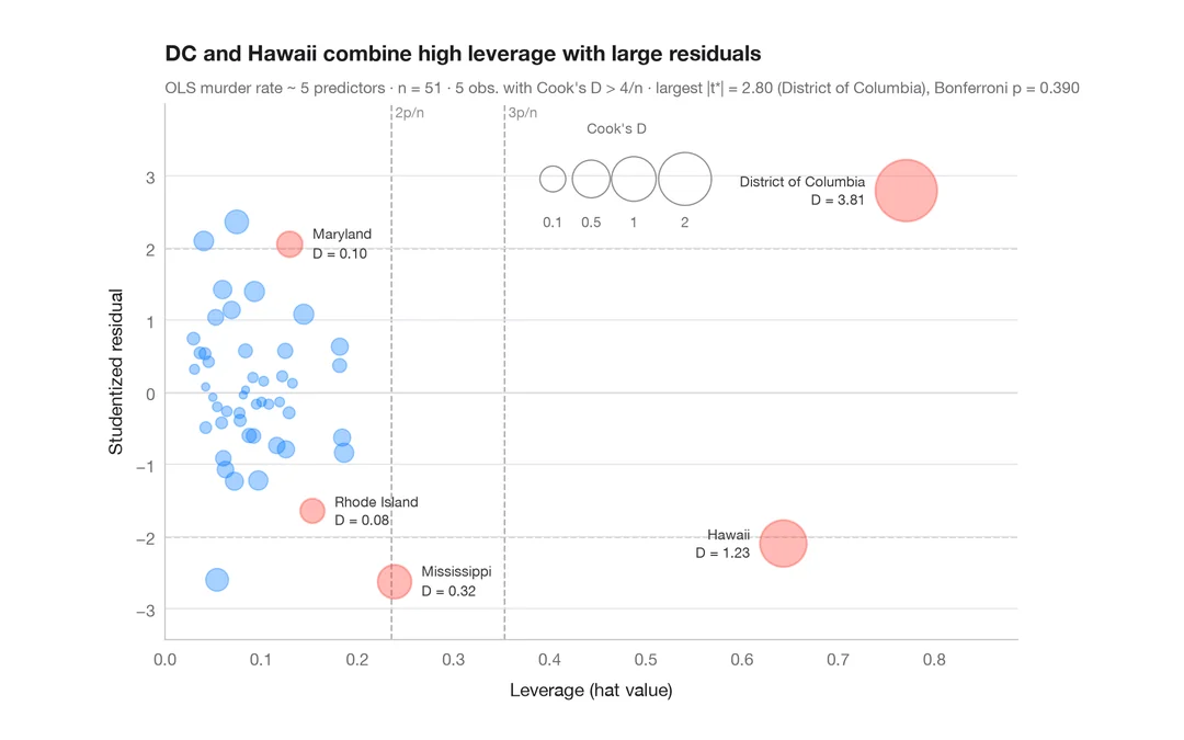
Influence plot
Studentized residuals vs leverage, with bubbles sized by Cook's distance.
car::influencePlot()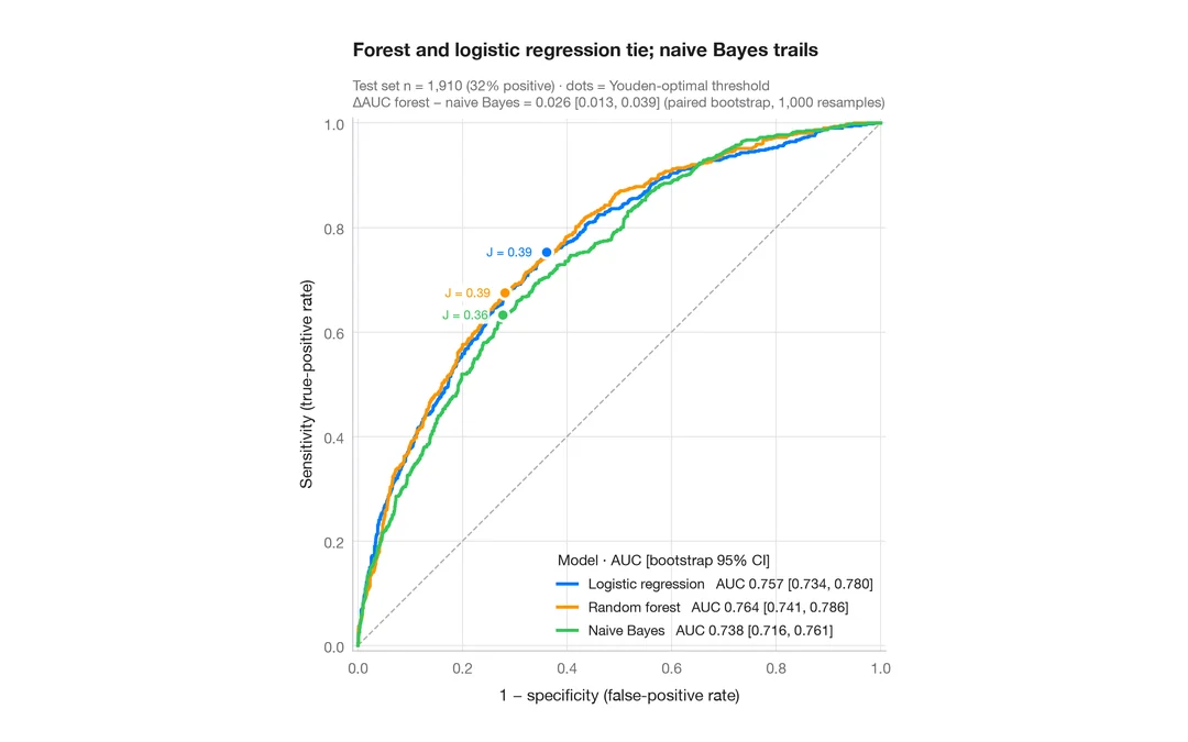
ROC curves
Three classifiers compared by ROC curve, AUC with bootstrap 95% CI and Youden point.
pROC::ggroc() / pROC::ci.auc()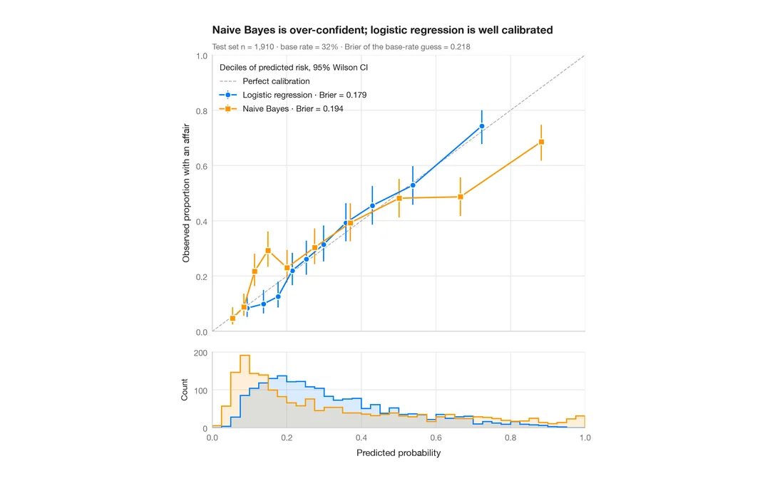
Calibration plot
Predicted vs observed risk per decile, with Wilson CIs, prediction histograms and Brier score.
rms::calibrate() / probably::cal_plot_breaks()