残差診断
線形モデルのための定番の 2 × 2 パネル。線形性、正規性、分散、てこ比を確認します。
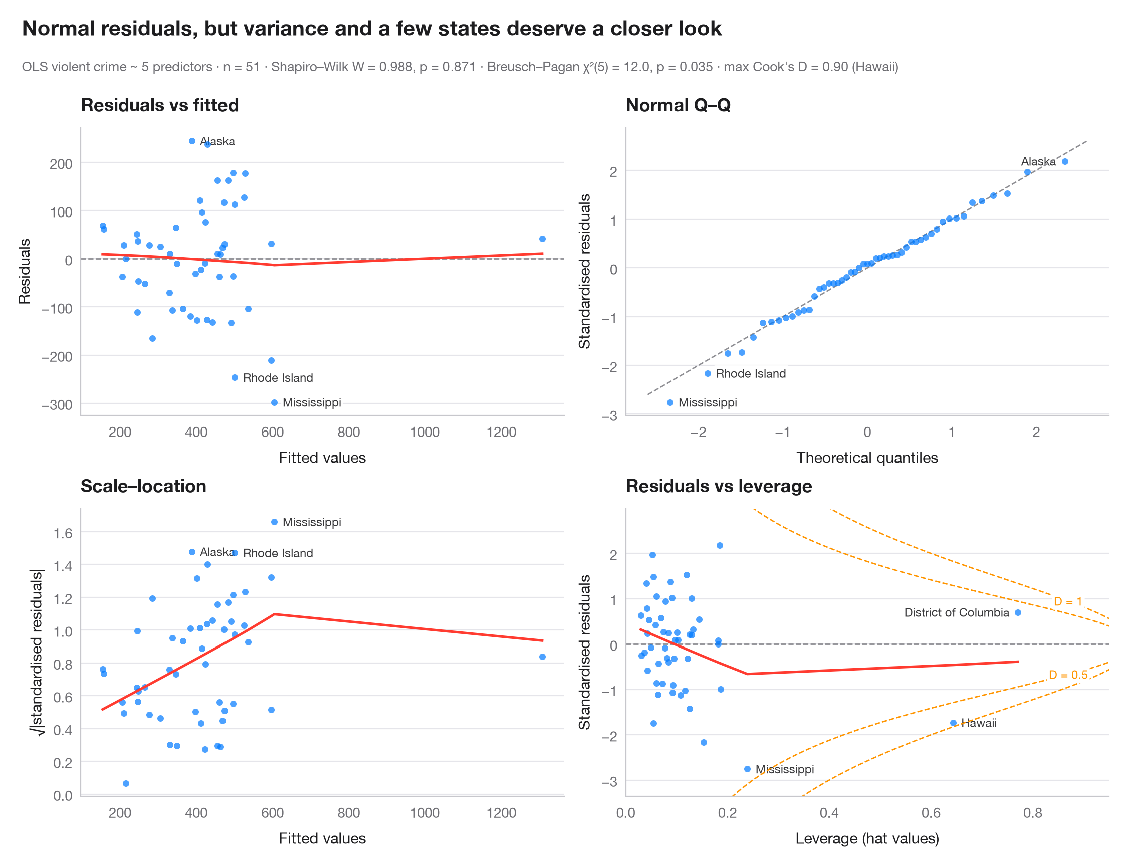
残差を4つの視点から見ることで、4つの問いに答えます。残差対予測値:関係は線形か(LOWESS 曲線が平坦か)。正規 Q–Q:残差はおおむね正規分布に従うか(点が直線上にあるか)。スケール・位置:ばらつきは一定か(曲線が平坦か)。残差対てこ比:当てはめを引っ張る観測値、すなわちクックの距離の破線の等高線の外側にある観測値はないか。各パネルでは最も極端な3つの観測値にラベルを付け、サブタイトルに正式な検定結果を示しています。
モデルは sm.datasets.statecrime の米国50州+DC を対象とした凶悪犯罪の回帰です。すべて statsmodels の get_influence() から求めており、平滑化には lowess() を、さらに het_breuschpagan() と scipy.stats.shapiro() を使用しています。
コードおよび図中のテキストは英語です。
import matplotlib.pyplot as plt
import numpy as np
import statsmodels.api as sm
import statsmodels.formula.api as smf
from scipy import stats
from statsmodels.nonparametric.smoothers_lowess import lowess
from statsmodels.stats.diagnostic import het_breuschpagan

df = sm.datasets.statecrime.load_pandas().data
model = smf.ols("violent ~ poverty + single + urban + hs_grad + white", data=df).fit()
infl = model.get_influence()
fitted, resid = model.fittedvalues, model.resid
std_r, lev, cook = infl.resid_studentized_internal, infl.hat_matrix_diag, infl.cooks_distance[0]
p = model.df_model + 1
top = np.argsort(-np.abs(std_r))[:3]                # 3 largest standardised residuals

fig, axes = plt.subplots(2, 2, figsize=(11, 7.6))
kw = dict(s=22, color="#007AFF", alpha=0.7, lw=0, zorder=2)
smooth = dict(color="#FF3B30", lw=1.8)

def label(ax, x, y, idx):
    lo, hi = ax.get_xlim()
    for i in idx:                                   # text on the side with more room
        right = (x[i] - lo) / (hi - lo) < 0.75
        ax.annotate(df.index[i], (x[i], y[i]), xytext=(6 if right else -6, 0),
                    textcoords="offset points", ha="left" if right else "right",
                    va="center", fontsize=8.5, color="#3A3A3C", zorder=1,
                    bbox=dict(boxstyle="round,pad=0.15", fc="white", ec="none", alpha=0.85))


# 1. Residuals vs fitted
ax = axes[0, 0]
ax.axhline(0, color="#8E8E93", lw=1, ls="--")
ax.scatter(fitted, resid, **kw)
ax.plot(*lowess(resid, fitted, frac=1, it=0).T, **smooth)
label(ax, fitted.values, resid.values, top)
ax.set(title="Residuals vs fitted", xlabel="Fitted values", ylabel="Residuals")

# 2. Normal Q-Q of standardised residuals
ax = axes[0, 1]
order = np.argsort(std_r)
theo = stats.norm.ppf((np.arange(1, len(std_r) + 1) - 0.5) / len(std_r))
ax.plot([-2.6, 2.6], [-2.6, 2.6], color="#8E8E93", lw=1, ls="--")
ax.scatter(theo, std_r[order], **kw)
rank = {i: k for k, i in enumerate(order)}
label(ax, {i: theo[rank[i]] for i in top}, std_r, top)
ax.set(title="Normal Q–Q", xlabel="Theoretical quantiles", ylabel="Standardised residuals")

# 3. Scale-location
ax = axes[1, 0]
root = np.sqrt(np.abs(std_r))
ax.scatter(fitted, root, **kw)
ax.plot(*lowess(root, fitted, frac=1, it=0).T, **smooth)
label(ax, fitted.values, np.abs(root), top)
ax.set(title="Scale–location", xlabel="Fitted values", ylabel="√|standardised residuals|")

# 4. Residuals vs leverage with Cook's distance contours
ax = axes[1, 1]
ax.axhline(0, color="#8E8E93", lw=1, ls="--")
ax.scatter(lev, std_r, **kw)
ax.plot(*lowess(std_r, lev, frac=1, it=0).T, **smooth)
ylim = (std_r.min() - 0.6, std_r.max() + 0.8)
h = np.linspace(0.01, 0.95, 300)
for D in (0.5, 1):
    r = np.sqrt(D * p * (1 - h) / h)
    ax.plot(h, r, color="#FF9500", lw=1, ls="--"); ax.plot(h, -r, color="#FF9500", lw=1, ls="--")
    sign = 1 if D == 1 else -1                       # label D = 1 above, D = 0.5 below
    ax.text(0.87, sign * np.sqrt(D * p * 0.13 / 0.87), f"D = {D}", color="#FF9500", fontsize=8.5,
            ha="center", va="center", bbox=dict(boxstyle="round,pad=0.15", fc="white", ec="none"))
ax.set_ylim(*ylim); ax.set_xlim(0, 0.95)
label(ax, lev, std_r, np.argsort(-cook)[:3])
ax.set(title="Residuals vs leverage", xlabel="Leverage (hat values)", ylabel="Standardised residuals")
for a in axes.flat:
    a.title.set_fontsize(12)

bp = het_breuschpagan(resid, model.model.exog)
sw = stats.shapiro(resid)
fig.text(0.01, 1.065, "Normal residuals, but variance and a few states deserve a closer look",
         fontsize=15, fontweight="semibold", va="bottom")
fig.text(0.01, 1.02, f"OLS violent crime ~ 5 predictors · n = {int(model.nobs)} · Shapiro–Wilk "
         f"W = {sw.statistic:.3f}, p = {sw.pvalue:.3f} · Breusch–Pagan χ²({p - 1:.0f}) = "
         f"{bp[0]:.1f}, p = {bp[1]:.3f} · max Cook's D = {cook.max():.2f} ({df.index[cook.argmax()]})",
         fontsize=9.5, color="#6E6E73", va="bottom")
plt.show()
図にはオプションの PyStatlas スタイル を使用しています。同じ見た目にするには plt.style.use("pystatlas.mplstyle") を追加してください。
データの出典
- US state crime and social indicators, 2009. U.S. Census Bureau. Statistical Abstract of the United States, state tables for 2009 (crime rates from the FBI Uniform Crime Reporting program). https://www.statsmodels.org/stable/datasets/generated/statecrime.html
Compiled for statsmodels (sm.datasets.statecrime); public domain. See the statsmodels page for each variable's table and footnotes.
これらの例は統計手法を説明するためのものです。図のタイトルは、この特定のデータ(多くは小規模で、古く、部分的な標本)で図が示す内容を述べたものであり、実質的な問いに対する著者の立場ではありません。解釈、背景、データの質については、ここに挙げた元の出典を参照してください。
引用方法
PyStatlas は Thierry Warin が作成・運営しています。研究や業務に役立った場合は、ぜひ引用してください。
Warin, T. (2026). Residual diagnostics. In PyStatlas: A Python Gallery of Statistical Graphics for the Social Sciences. https://warint.github.io/pystatlas/model-diagnostics/residual-diagnostics/
@misc{warin2026statlas,
  author       = {Warin, Thierry},
  title        = {PyStatlas: A Python Gallery of Statistical Graphics for the Social Sciences},
  year         = {2026},
  howpublished = {\url{https://warint.github.io/pystatlas/}},
  note         = {Source code: https://github.com/warint/pystatlas}
}