キャリブレーションプロット
十分位ごとの予測リスク対観測リスクを、ウィルソン信頼区間、予測値のヒストグラム、ブライアスコアとともに示します。
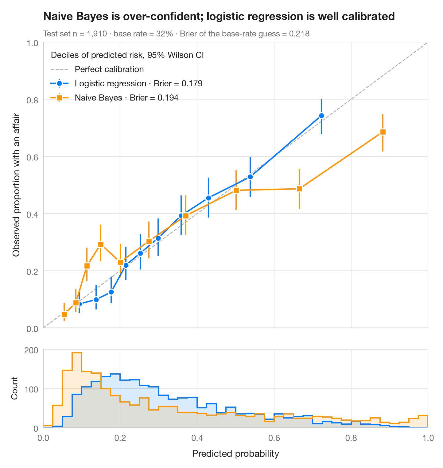
モデルは事例をうまく順位付けできても(AUC が高くても)、誤った確率を出すことがあります。信頼性ダイアグラムはこれを確認するためのものです。テスト事例を予測リスクの十分位でグループ分けし、各ビンの平均予測値を観測されたイベント発生率に対して 95% ウィルソン区間とともにプロットします。較正の取れたモデルは対角線上に並び、対角線より下の点はモデルが過信していることを意味します。下のヒストグラムは、予測値が実際にどこに分布しているかを示しています。
データはフェアの婚外関係調査(sm.datasets.fair)で、70/30 に分割しています。scikit-learn のロジスティック回帰とガウシアン・ナイーブベイズのモデルを比較し、ブライアスコア(brier_score_loss、小さいほど良い)で確率の精度を要約しています。区間は proportion_confint(method="wilson") で求めています。
コードおよび図中のテキストは英語です。
import matplotlib.pyplot as plt
import numpy as np
import pandas as pd
import statsmodels.api as sm
from sklearn.linear_model import LogisticRegression
from sklearn.metrics import brier_score_loss
from sklearn.model_selection import train_test_split
from sklearn.naive_bayes import GaussianNB
from statsmodels.stats.proportion import proportion_confint

df = sm.datasets.fair.load_pandas().data
X, y = df.drop(columns="affairs").to_numpy(), (df.affairs > 0).astype(int).to_numpy()
X_tr, X_te, y_tr, y_te = train_test_split(X, y, test_size=0.3, stratify=y, random_state=1)
models = {"Logistic regression": (LogisticRegression(max_iter=1000), "#007AFF", "o"),
          "Naive Bayes": (GaussianNB(), "#FF9500", "s")}

fig, (ax, axh) = plt.subplots(2, 1, figsize=(7, 7.4), sharex=True,
                              gridspec_kw=dict(height_ratios=[4, 1.1], hspace=0.05))
ax.plot([0, 1], [0, 1], color="#AEAEB2", lw=1, ls="--", label="Perfect calibration")
bins = np.linspace(0, 1, 41)
for name, (clf, c, mk) in models.items():
    p = clf.fit(X_tr, y_tr).predict_proba(X_te)[:, 1]
    # Group predictions into deciles of predicted risk
    tab = (pd.DataFrame({"p": p, "y": y_te})
             .assign(bin=lambda d: pd.qcut(d.p, 10, labels=False, duplicates="drop"))
             .groupby("bin").agg(pred=("p", "mean"), obs=("y", "mean"), k=("y", "sum"), n=("y", "size")))
    lo, hi = proportion_confint(tab.k, tab.n, method="wilson")
    ax.errorbar(tab.pred, tab.obs, yerr=[tab.obs - lo, hi - tab.obs], fmt=mk + "-", color=c,
                ms=7, mec="white", mew=1.2, lw=1.6, capsize=0, elinewidth=1.4,
                label=f"{name} · Brier = {brier_score_loss(y_te, p):.3f}")
    axh.hist(p, bins=bins, color=c, alpha=0.15, lw=0)
    axh.hist(p, bins=bins, color=c, histtype="step", lw=1.4)

ax.set_xlim(0, 1); ax.set_ylim(0, 1); ax.set_aspect("auto")
ax.grid(axis="x")
ax.set_ylabel("Observed proportion with an affair")
ax.legend(loc="upper left", alignment="left", title="Deciles of predicted risk, 95% Wilson CI")
axh.set_xlabel("Predicted probability")
axh.set_ylabel("Count", fontsize=10)
axh.grid(axis="x")
ax.set_title("Naive Bayes is over-confident; logistic regression is well calibrated", pad=26)
ax.text(0, 1.02, f"Test set n = {len(y_te):,} · base rate = {y_te.mean():.0%} · "
        f"Brier of the base-rate guess = {y_te.mean() * (1 - y_te.mean()):.3f}",
        transform=ax.transAxes, fontsize=9.5, color="#6E6E73")
plt.show()
図にはオプションの PyStatlas スタイル を使用しています。同じ見た目にするには plt.style.use("pystatlas.mplstyle") を追加してください。
データの出典
- Redbook survey of married women, 1974 (Fair's affairs data). Fair, R. C. (1978). A theory of extramarital affairs. Journal of Political Economy, 86(1), 45–61. https://doi.org/10.1086/260646
Data from the 1974 Redbook magazine survey; distributed with statsmodels (sm.datasets.fair) with the author's permission.
これらの例は統計手法を説明するためのものです。図のタイトルは、この特定のデータ(多くは小規模で、古く、部分的な標本)で図が示す内容を述べたものであり、実質的な問いに対する著者の立場ではありません。解釈、背景、データの質については、ここに挙げた元の出典を参照してください。
引用方法
PyStatlas は Thierry Warin が作成・運営しています。研究や業務に役立った場合は、ぜひ引用してください。
Warin, T. (2026). Calibration plot. In PyStatlas: A Python Gallery of Statistical Graphics for the Social Sciences. https://warint.github.io/pystatlas/model-diagnostics/calibration-plot/
@misc{warin2026statlas,
  author       = {Warin, Thierry},
  title        = {PyStatlas: A Python Gallery of Statistical Graphics for the Social Sciences},
  year         = {2026},
  howpublished = {\url{https://warint.github.io/pystatlas/}},
  note         = {Source code: https://github.com/warint/pystatlas}
}