Added-variable plots — PyStatlas: A Python Gallery of Statistical Graphics for the Social Sciences

Warin, Thierry

追加変数プロット

説明変数ごとの偏回帰パネル。当てはめた各傾きはその回帰係数に一致します。

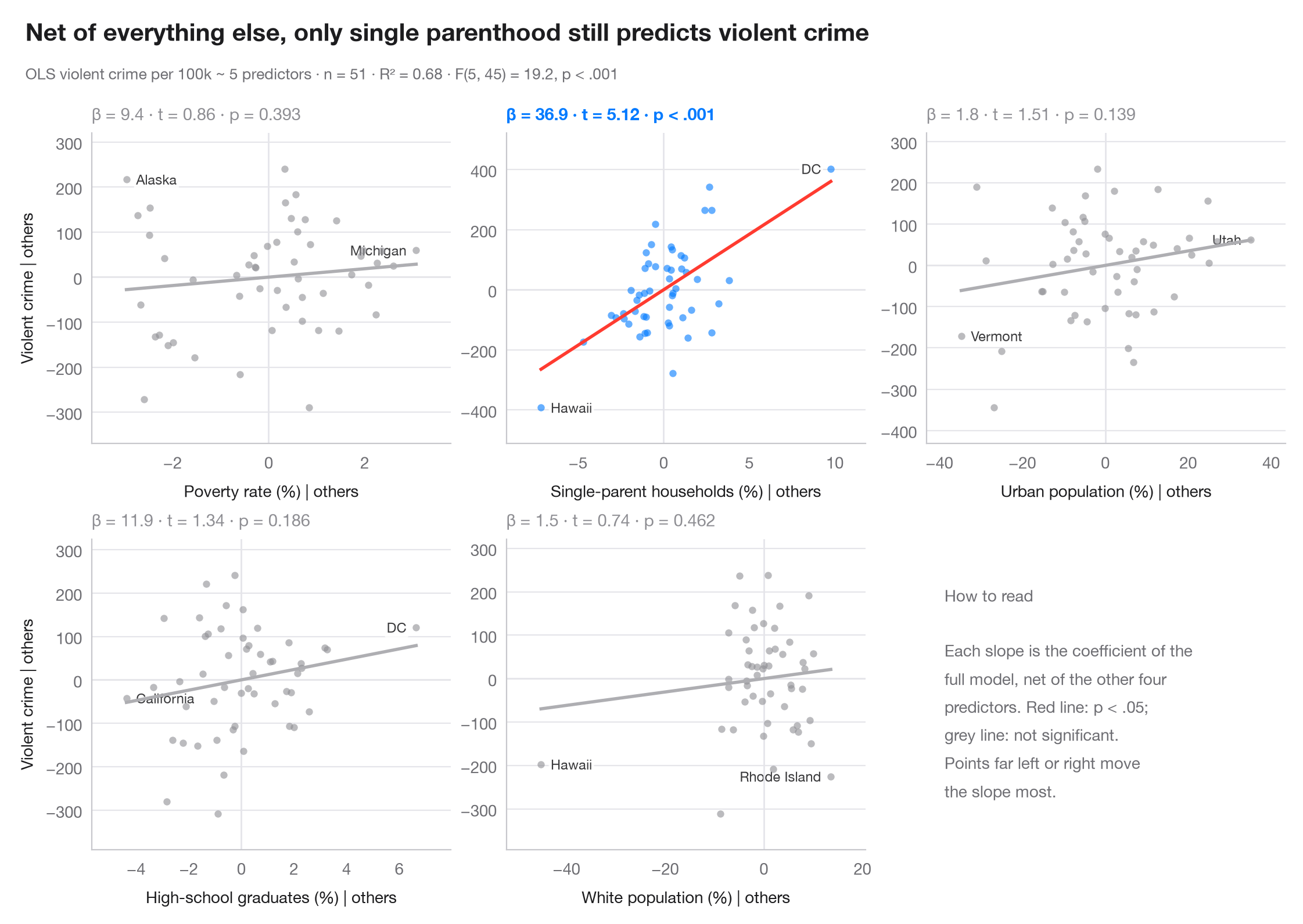
重回帰では、y と1つの説明変数の単純な散布図には、その変数の効果と、それに相関するあらゆるものの効果が混在します。追加変数プロット はこれを取り除きます。y を他のすべての説明変数に回帰した残差を、注目する説明変数を同じ説明変数に回帰した残差に対してプロットするのです。フリッシュ・ウォー・ロヴェルの定理により、点群を通る直線の傾きは重回帰係数にちょうど一致し、x軸上で遠く離れた点がその係数を左右している点です。

モデルは sm.datasets.statecrime の米国50州＋DC を対象とした凶悪犯罪の回帰で、statsmodels の smf.ols() で当てはめています。残差は軸ごとに1回の補助的な OLS で計算し、各パネルに β とその t 値、p値を示しています。

コードおよび図中のテキストは英語です。

partial-regression.py · 54 行

ダウンロード GitHub

import matplotlib.pyplot as plt
import numpy as np
import statsmodels.api as sm
import statsmodels.formula.api as smf

df = sm.datasets.statecrime.load_pandas().data
predictors = ["poverty", "single", "urban", "hs_grad", "white"]
labels = {"poverty": "Poverty rate (%)", "single": "Single-parent households (%)",
          "urban": "Urban population (%)", "hs_grad": "High-school graduates (%)",
          "white": "White population (%)"}
full = smf.ols("violent ~ " + " + ".join(predictors), data=df).fit()

fig, axes = plt.subplots(2, 3, figsize=(11, 7))
for ax, x in zip(axes.flat, predictors):
    others = " + ".join(p for p in predictors if p != x)
    ey = smf.ols(f"violent ~ {others}", data=df).fit().resid      # y | others
    ex = smf.ols(f"{x} ~ {others}", data=df).fit().resid          # x | others
    sig = full.pvalues[x] < 0.05
    c = "#007AFF" if sig else "#8E8E93"

    ax.axhline(0, color="#E5E5EA", lw=1); ax.axvline(0, color="#E5E5EA", lw=1)
    ax.scatter(ex, ey, s=20, color=c, alpha=0.6, lw=0, zorder=2)
    grid = np.linspace(ex.min(), ex.max(), 2)
    ax.plot(grid, full.params[x] * grid, color="#FF3B30" if sig else "#AEAEB2", lw=2)
    # Label the two observations with the most extreme partial x
    for i in np.argsort(-np.abs(ex.to_numpy()))[:2]:
        right = ex.iloc[i] < 0
        ax.annotate(df.index[i].replace("District of Columbia", "DC"), (ex.iloc[i], ey.iloc[i]),
                    xytext=(6 if right else -6, 0), textcoords="offset points",
                    ha="left" if right else "right", va="center", fontsize=8.5, color="#3A3A3C",
                    zorder=1, bbox=dict(boxstyle="round,pad=0.15", fc="white", ec="none", alpha=0.85))
    p = full.pvalues[x]
    ax.set_title(f"β = {full.params[x]:.1f} · t = {full.tvalues[x]:.2f} · "
                 + ("p < .001" if p < .001 else f"p = {p:.3f}"), fontsize=10.5, color=c,
                 fontweight="semibold" if sig else "normal", pad=8)
    ax.set_xlabel(f"{labels[x]} | others", fontsize=10)
    if ax.get_subplotspec().is_first_col():
        ax.set_ylabel("Violent crime | others", fontsize=10)
    ax.margins(x=0.12, y=0.15)

# Last cell: reading guide instead of an empty panel
axes.flat[-1].axis("off")
axes.flat[-1].text(0.05, 0.5, "How to read\n\nEach slope is the coefficient of the\n"
                   "full model, net of the other four\npredictors. Red line: p < .05;\n"
                   "grey line: not significant.\nPoints far left or right move\n"
                   "the slope most.", transform=axes.flat[-1].transAxes, va="center",
                   fontsize=10, color="#6E6E73", linespacing=1.5)

fig.text(0.01, 1.065, "Net of everything else, only single parenthood still predicts violent crime",
         fontsize=15, fontweight="semibold", va="bottom")
fig.text(0.01, 1.02, f"OLS violent crime per 100k ~ 5 predictors · n = {int(full.nobs)} · "
         f"R² = {full.rsquared:.2f} · F({full.df_model:.0f}, {full.df_resid:.0f}) = "
         f"{full.fvalue:.1f}, p < .001", fontsize=9.5, color="#6E6E73", va="bottom")
plt.show()

図にはオプションの PyStatlas スタイルを使用しています。同じ見た目にするには plt.style.use("pystatlas.mplstyle") を追加してください。

データの出典

US state crime and social indicators, 2009. U.S. Census Bureau. Statistical Abstract of the United States, state tables for 2009 (crime rates from the FBI Uniform Crime Reporting program). https://www.statsmodels.org/stable/datasets/generated/statecrime.html
Compiled for statsmodels (sm.datasets.statecrime); public domain. See the statsmodels page for each variable's table and footnotes.

これらの例は統計手法を説明するためのものです。図のタイトルは、この特定のデータ（多くは小規模で、古く、部分的な標本）で図が示す内容を述べたものであり、実質的な問いに対する著者の立場ではありません。解釈、背景、データの質については、ここに挙げた元の出典を参照してください。

引用方法

PyStatlas は Thierry Warin が作成・運営しています。研究や業務に役立った場合は、ぜひ引用してください。

Warin, T. (2026). Added-variable plots. In PyStatlas: A Python Gallery of Statistical Graphics for the Social Sciences. https://warint.github.io/pystatlas/model-diagnostics/partial-regression/

@misc{warin2026statlas,
  author       = {Warin, Thierry},
  title        = {PyStatlas: A Python Gallery of Statistical Graphics for the Social Sciences},
  year         = {2026},
  howpublished = {\url{https://warint.github.io/pystatlas/}},
  note         = {Source code: https://github.com/warint/pystatlas}
}