Added-variable plots
One partial-regression panel per predictor; each fitted slope equals its coefficient.
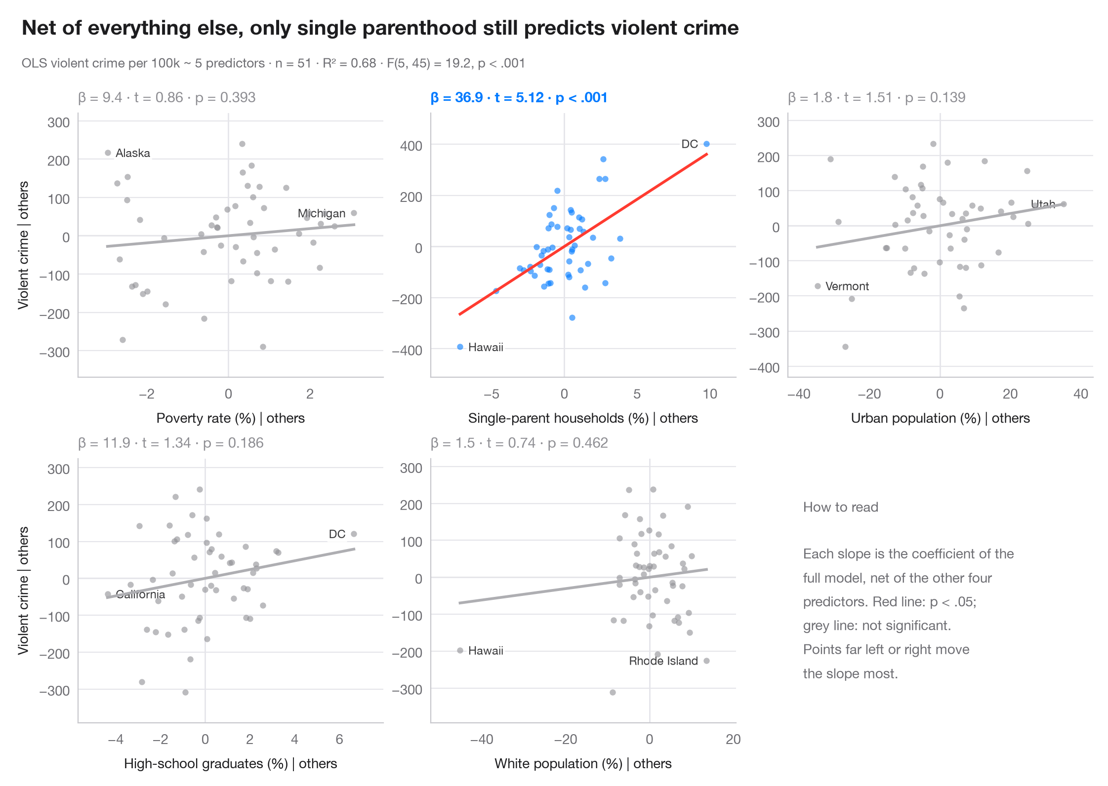
In a multiple regression, a raw scatter of y against one predictor mixes its effect with everything correlated with it. An added-variable plot removes that: it plots the residuals of y on all other predictors against the residuals of the focal predictor on those same predictors. By the Frisch–Waugh–Lovell theorem, the slope of the line through the cloud is exactly the multiple-regression coefficient, and points far out on the x-axis are the ones that drive that coefficient.
The model is the violent-crime regression on the 50 US states + DC from
sm.datasets.statecrime, fitted with statsmodels smf.ols(). Residuals are
computed with one auxiliary OLS fit per axis; each panel reports β, its t and p.
import matplotlib.pyplot as plt
import numpy as np
import statsmodels.api as sm
import statsmodels.formula.api as smf

df = sm.datasets.statecrime.load_pandas().data
predictors = ["poverty", "single", "urban", "hs_grad", "white"]
labels = {"poverty": "Poverty rate (%)", "single": "Single-parent households (%)",
          "urban": "Urban population (%)", "hs_grad": "High-school graduates (%)",
          "white": "White population (%)"}
full = smf.ols("violent ~ " + " + ".join(predictors), data=df).fit()

fig, axes = plt.subplots(2, 3, figsize=(11, 7))
for ax, x in zip(axes.flat, predictors):
    others = " + ".join(p for p in predictors if p != x)
    ey = smf.ols(f"violent ~ {others}", data=df).fit().resid      # y | others
    ex = smf.ols(f"{x} ~ {others}", data=df).fit().resid          # x | others
    sig = full.pvalues[x] < 0.05
    c = "#007AFF" if sig else "#8E8E93"

    ax.axhline(0, color="#E5E5EA", lw=1); ax.axvline(0, color="#E5E5EA", lw=1)
    ax.scatter(ex, ey, s=20, color=c, alpha=0.6, lw=0, zorder=2)
    grid = np.linspace(ex.min(), ex.max(), 2)
    ax.plot(grid, full.params[x] * grid, color="#FF3B30" if sig else "#AEAEB2", lw=2)
    # Label the two observations with the most extreme partial x
    for i in np.argsort(-np.abs(ex.to_numpy()))[:2]:
        right = ex.iloc[i] < 0
        ax.annotate(df.index[i].replace("District of Columbia", "DC"), (ex.iloc[i], ey.iloc[i]),
                    xytext=(6 if right else -6, 0), textcoords="offset points",
                    ha="left" if right else "right", va="center", fontsize=8.5, color="#3A3A3C",
                    zorder=1, bbox=dict(boxstyle="round,pad=0.15", fc="white", ec="none", alpha=0.85))
    p = full.pvalues[x]
    ax.set_title(f"β = {full.params[x]:.1f} · t = {full.tvalues[x]:.2f} · "
                 + ("p < .001" if p < .001 else f"p = {p:.3f}"), fontsize=10.5, color=c,
                 fontweight="semibold" if sig else "normal", pad=8)
    ax.set_xlabel(f"{labels[x]} | others", fontsize=10)
    if ax.get_subplotspec().is_first_col():
        ax.set_ylabel("Violent crime | others", fontsize=10)
    ax.margins(x=0.12, y=0.15)

# Last cell: reading guide instead of an empty panel
axes.flat[-1].axis("off")
axes.flat[-1].text(0.05, 0.5, "How to read\n\nEach slope is the coefficient of the\n"
                   "full model, net of the other four\npredictors. Red line: p < .05;\n"
                   "grey line: not significant.\nPoints far left or right move\n"
                   "the slope most.", transform=axes.flat[-1].transAxes, va="center",
                   fontsize=10, color="#6E6E73", linespacing=1.5)

fig.text(0.01, 1.065, "Net of everything else, only single parenthood still predicts violent crime",
         fontsize=15, fontweight="semibold", va="bottom")
fig.text(0.01, 1.02, f"OLS violent crime per 100k ~ 5 predictors · n = {int(full.nobs)} · "
         f"R² = {full.rsquared:.2f} · F({full.df_model:.0f}, {full.df_resid:.0f}) = "
         f"{full.fvalue:.1f}, p < .001", fontsize=9.5, color="#6E6E73", va="bottom")
plt.show()
Figures use the optional PyStatlas style: add plt.style.use("pystatlas.mplstyle") to match the look exactly.
Data source
- US state crime and social indicators, 2009. U.S. Census Bureau. Statistical Abstract of the United States, state tables for 2009 (crime rates from the FBI Uniform Crime Reporting program). https://www.statsmodels.org/stable/datasets/generated/statecrime.html
Compiled for statsmodels (sm.datasets.statecrime); public domain. See the statsmodels page for each variable's table and footnotes.
The examples illustrate statistical methods. Their titles describe what each figure shows in these particular data — often a small, dated or partial sample — not the author's position on the substantive question. For interpretation, context and data quality, rely on the original sources cited here.
How to cite
PyStatlas is created and maintained by Thierry Warin. If it helped your work, please cite it.
Warin, T. (2026). Added-variable plots. In PyStatlas: A Python Gallery of Statistical Graphics for the Social Sciences. https://warint.github.io/pystatlas/model-diagnostics/partial-regression/
@misc{warin2026statlas,
  author       = {Warin, Thierry},
  title        = {PyStatlas: A Python Gallery of Statistical Graphics for the Social Sciences},
  year         = {2026},
  howpublished = {\url{https://warint.github.io/pystatlas/}},
  note         = {Source code: https://github.com/warint/pystatlas}
}More in Model diagnostics
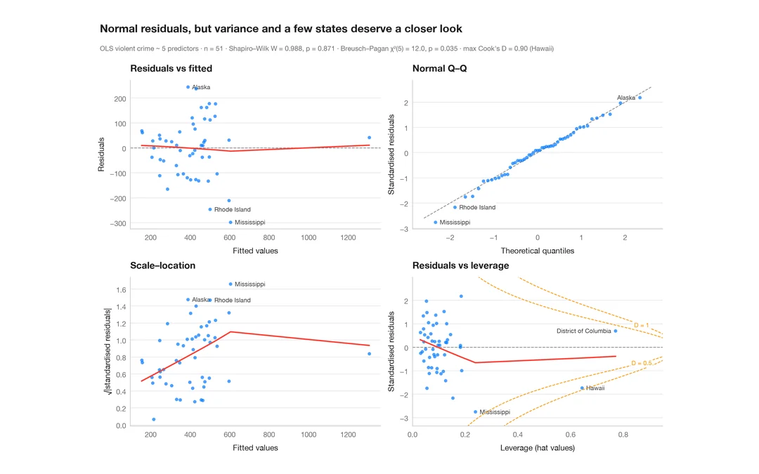
Residual diagnostics
The classic 2 × 2 panel for a linear model — linearity, normality, variance, leverage.
plot(lm) / performance::check_model()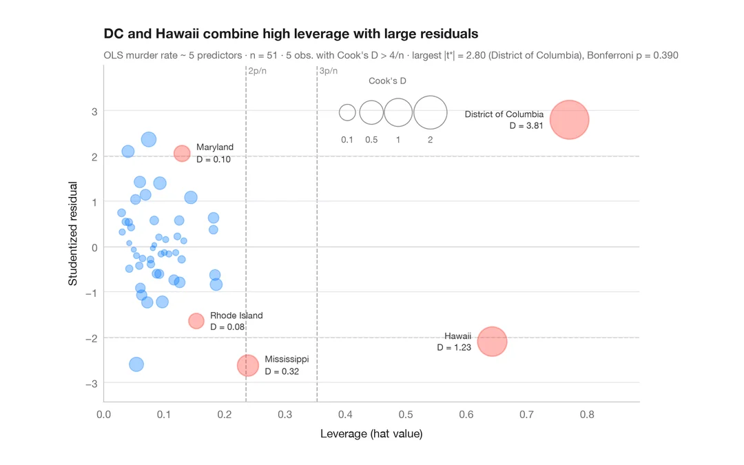
Influence plot
Studentized residuals vs leverage, with bubbles sized by Cook's distance.
car::influencePlot()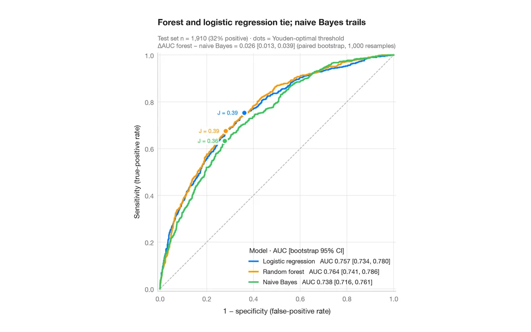
ROC curves
Three classifiers compared by ROC curve, AUC with bootstrap 95% CI and Youden point.
pROC::ggroc() / pROC::ci.auc()