Graphiques de variables ajoutées
Un panneau de régression partielle par prédicteur ; chaque pente ajustée est égale à son coefficient.
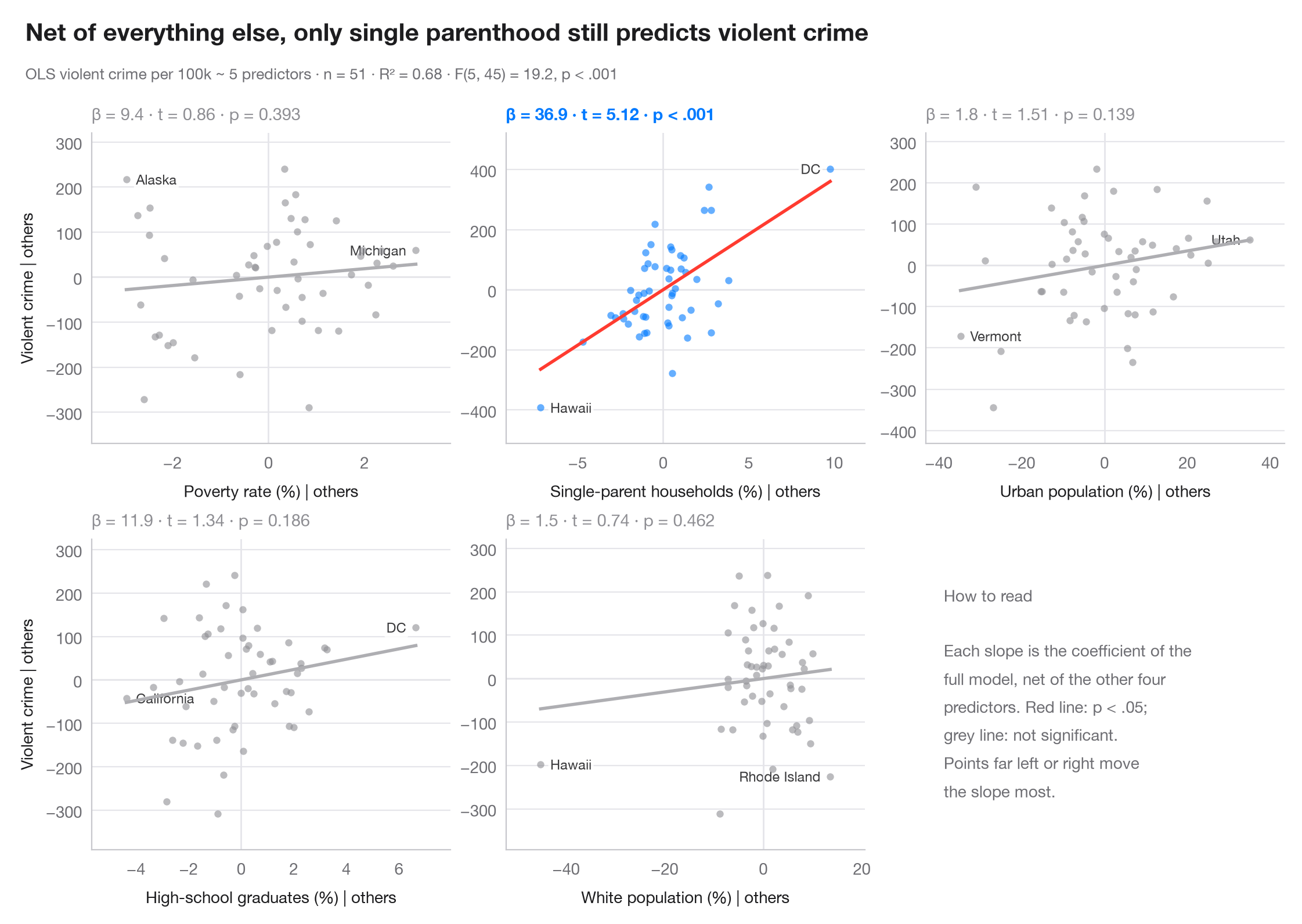
Dans une régression multiple, un simple nuage de y en fonction d'un prédicteur mélange son effet avec celui de tout ce qui lui est corrélé. Un graphique de variable ajoutée élimine ce mélange : il met en regard les résidus de y sur tous les autres prédicteurs et les résidus du prédicteur focal sur ces mêmes prédicteurs. D'après le théorème de Frisch–Waugh–Lovell, la pente de la droite qui traverse le nuage est exactement le coefficient de la régression multiple, et les points éloignés sur l'axe des x sont ceux qui déterminent ce coefficient.
Le modèle est la régression des crimes violents sur les 50 États américains + DC, tirée de sm.datasets.statecrime et ajustée avec smf.ols() de statsmodels. Les résidus sont calculés à l'aide d'un ajustement MCO auxiliaire par axe ; chaque panneau rapporte β, son t et sa valeur p.
Le code et le texte à l'intérieur des figures sont en anglais.
import matplotlib.pyplot as plt
import numpy as np
import statsmodels.api as sm
import statsmodels.formula.api as smf

df = sm.datasets.statecrime.load_pandas().data
predictors = ["poverty", "single", "urban", "hs_grad", "white"]
labels = {"poverty": "Poverty rate (%)", "single": "Single-parent households (%)",
          "urban": "Urban population (%)", "hs_grad": "High-school graduates (%)",
          "white": "White population (%)"}
full = smf.ols("violent ~ " + " + ".join(predictors), data=df).fit()

fig, axes = plt.subplots(2, 3, figsize=(11, 7))
for ax, x in zip(axes.flat, predictors):
    others = " + ".join(p for p in predictors if p != x)
    ey = smf.ols(f"violent ~ {others}", data=df).fit().resid      # y | others
    ex = smf.ols(f"{x} ~ {others}", data=df).fit().resid          # x | others
    sig = full.pvalues[x] < 0.05
    c = "#007AFF" if sig else "#8E8E93"

    ax.axhline(0, color="#E5E5EA", lw=1); ax.axvline(0, color="#E5E5EA", lw=1)
    ax.scatter(ex, ey, s=20, color=c, alpha=0.6, lw=0, zorder=2)
    grid = np.linspace(ex.min(), ex.max(), 2)
    ax.plot(grid, full.params[x] * grid, color="#FF3B30" if sig else "#AEAEB2", lw=2)
    # Label the two observations with the most extreme partial x
    for i in np.argsort(-np.abs(ex.to_numpy()))[:2]:
        right = ex.iloc[i] < 0
        ax.annotate(df.index[i].replace("District of Columbia", "DC"), (ex.iloc[i], ey.iloc[i]),
                    xytext=(6 if right else -6, 0), textcoords="offset points",
                    ha="left" if right else "right", va="center", fontsize=8.5, color="#3A3A3C",
                    zorder=1, bbox=dict(boxstyle="round,pad=0.15", fc="white", ec="none", alpha=0.85))
    p = full.pvalues[x]
    ax.set_title(f"β = {full.params[x]:.1f} · t = {full.tvalues[x]:.2f} · "
                 + ("p < .001" if p < .001 else f"p = {p:.3f}"), fontsize=10.5, color=c,
                 fontweight="semibold" if sig else "normal", pad=8)
    ax.set_xlabel(f"{labels[x]} | others", fontsize=10)
    if ax.get_subplotspec().is_first_col():
        ax.set_ylabel("Violent crime | others", fontsize=10)
    ax.margins(x=0.12, y=0.15)

# Last cell: reading guide instead of an empty panel
axes.flat[-1].axis("off")
axes.flat[-1].text(0.05, 0.5, "How to read\n\nEach slope is the coefficient of the\n"
                   "full model, net of the other four\npredictors. Red line: p < .05;\n"
                   "grey line: not significant.\nPoints far left or right move\n"
                   "the slope most.", transform=axes.flat[-1].transAxes, va="center",
                   fontsize=10, color="#6E6E73", linespacing=1.5)

fig.text(0.01, 1.065, "Net of everything else, only single parenthood still predicts violent crime",
         fontsize=15, fontweight="semibold", va="bottom")
fig.text(0.01, 1.02, f"OLS violent crime per 100k ~ 5 predictors · n = {int(full.nobs)} · "
         f"R² = {full.rsquared:.2f} · F({full.df_model:.0f}, {full.df_resid:.0f}) = "
         f"{full.fvalue:.1f}, p < .001", fontsize=9.5, color="#6E6E73", va="bottom")
plt.show()
Les figures utilisent le style PyStatlas (facultatif) : ajoutez plt.style.use("pystatlas.mplstyle") pour obtenir exactement le même rendu.
Source des données
- US state crime and social indicators, 2009. U.S. Census Bureau. Statistical Abstract of the United States, state tables for 2009 (crime rates from the FBI Uniform Crime Reporting program). https://www.statsmodels.org/stable/datasets/generated/statecrime.html
Compiled for statsmodels (sm.datasets.statecrime); public domain. See the statsmodels page for each variable's table and footnotes.
Les exemples illustrent des méthodes statistiques. Leurs titres décrivent ce que chaque figure montre dans ces données précises — souvent un échantillon restreint, daté ou partiel —, et non la position de l'auteur sur la question de fond. Pour l'interprétation, le contexte et la qualité des données, reportez-vous aux sources originales citées ici.
Comment citer
PyStatlas est créé et maintenu par Thierry Warin. S'il vous a été utile dans vos travaux, merci de le citer.
Warin, T. (2026). Added-variable plots. In PyStatlas: A Python Gallery of Statistical Graphics for the Social Sciences. https://warint.github.io/pystatlas/model-diagnostics/partial-regression/
@misc{warin2026statlas,
  author       = {Warin, Thierry},
  title        = {PyStatlas: A Python Gallery of Statistical Graphics for the Social Sciences},
  year         = {2026},
  howpublished = {\url{https://warint.github.io/pystatlas/}},
  note         = {Source code: https://github.com/warint/pystatlas}
}Plus dans Diagnostics de modèles
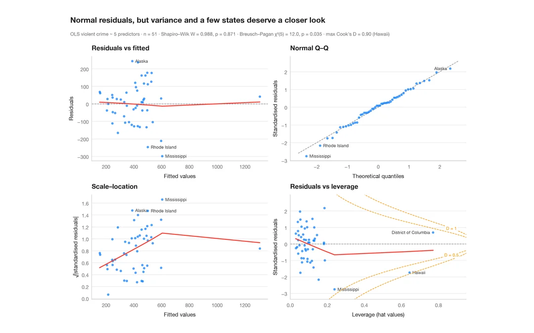
Diagnostics des résidus
Le panneau classique 2 × 2 d'un modèle linéaire — linéarité, normalité, variance, effet de levier.
plot(lm) / performance::check_model()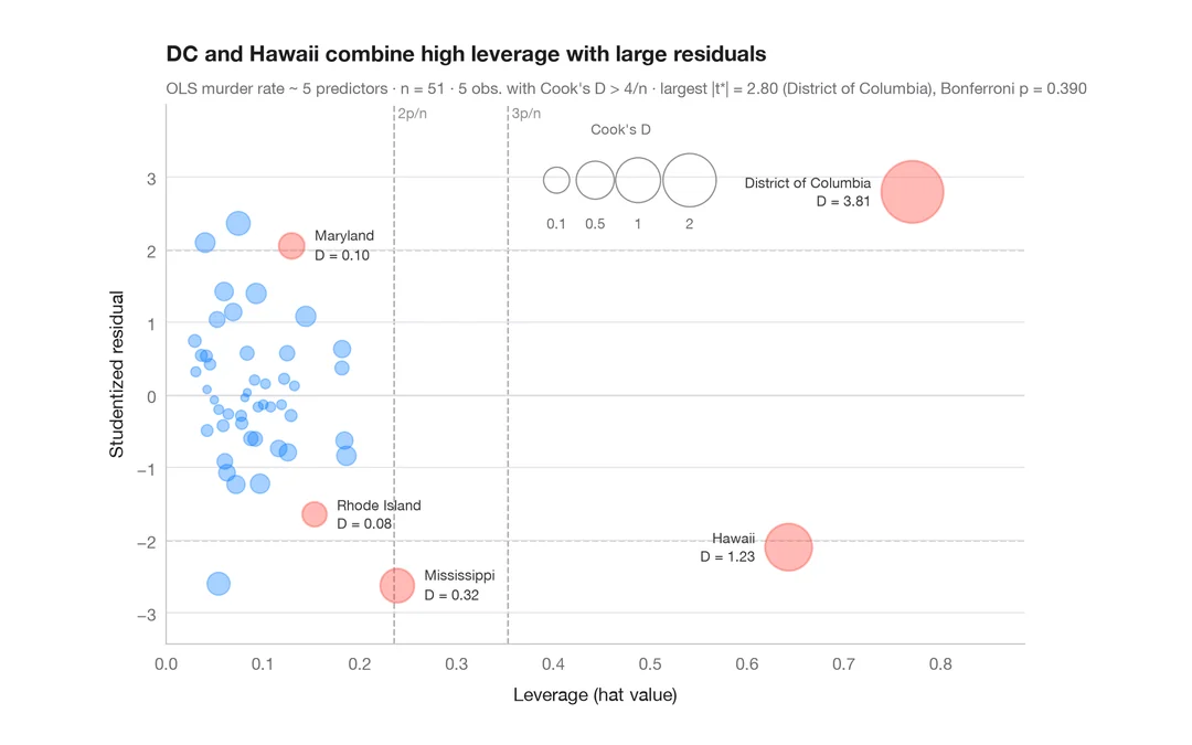
Graphique d'influence
Résidus studentisés en fonction de l'effet de levier, avec des bulles proportionnelles à la distance de Cook.
car::influencePlot()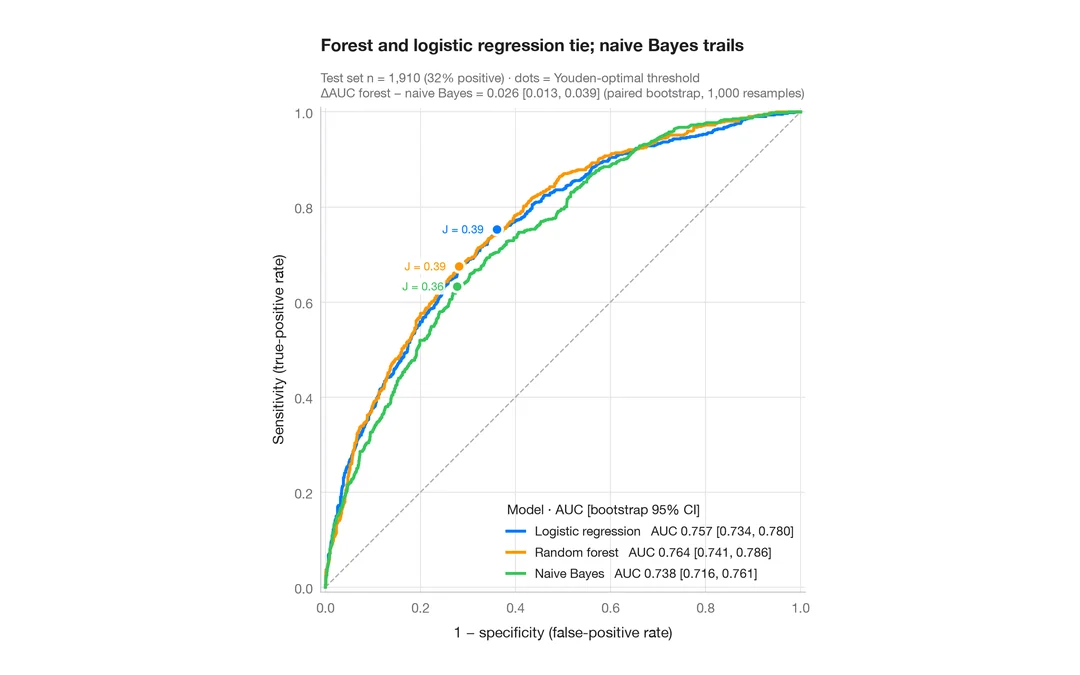
Courbes ROC
Trois classificateurs comparés par courbe ROC, AUC avec IC à 95 % par bootstrap et point de Youden.
pROC::ggroc() / pROC::ci.auc()