添加变量图
每个预测变量一张偏回归图;每条拟合斜率都等于对应的回归系数。
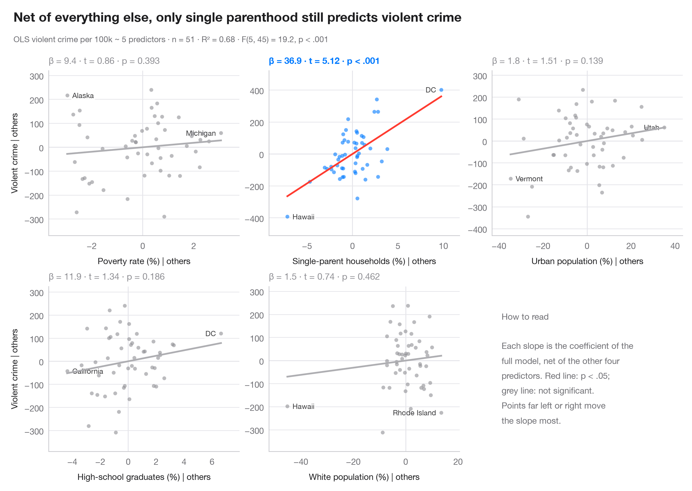
在多元回归中,y 对单个预测变量的原始散点图会把该变量的效应与所有与之相关的因素混在一起。添加变量图消除了这种混杂:它将 y 对所有其他预测变量回归的残差,与焦点预测变量对同样这些预测变量回归的残差相对照。根据 Frisch–Waugh–Lovell 定理,穿过点云的直线斜率恰好等于多元回归系数,而在 x 轴上远离中心的点正是驱动该系数的观测值。
模型是基于 sm.datasets.statecrime 中美国 50 个州 + 哥伦比亚特区的暴力犯罪回归,用 statsmodels smf.ols() 拟合。残差由每个坐标轴各一次辅助 OLS 拟合计算;每个子图报告 β 及其 t 值和 p 值。
代码及图中文字均为英文。
import matplotlib.pyplot as plt
import numpy as np
import statsmodels.api as sm
import statsmodels.formula.api as smf

df = sm.datasets.statecrime.load_pandas().data
predictors = ["poverty", "single", "urban", "hs_grad", "white"]
labels = {"poverty": "Poverty rate (%)", "single": "Single-parent households (%)",
          "urban": "Urban population (%)", "hs_grad": "High-school graduates (%)",
          "white": "White population (%)"}
full = smf.ols("violent ~ " + " + ".join(predictors), data=df).fit()

fig, axes = plt.subplots(2, 3, figsize=(11, 7))
for ax, x in zip(axes.flat, predictors):
    others = " + ".join(p for p in predictors if p != x)
    ey = smf.ols(f"violent ~ {others}", data=df).fit().resid      # y | others
    ex = smf.ols(f"{x} ~ {others}", data=df).fit().resid          # x | others
    sig = full.pvalues[x] < 0.05
    c = "#007AFF" if sig else "#8E8E93"

    ax.axhline(0, color="#E5E5EA", lw=1); ax.axvline(0, color="#E5E5EA", lw=1)
    ax.scatter(ex, ey, s=20, color=c, alpha=0.6, lw=0, zorder=2)
    grid = np.linspace(ex.min(), ex.max(), 2)
    ax.plot(grid, full.params[x] * grid, color="#FF3B30" if sig else "#AEAEB2", lw=2)
    # Label the two observations with the most extreme partial x
    for i in np.argsort(-np.abs(ex.to_numpy()))[:2]:
        right = ex.iloc[i] < 0
        ax.annotate(df.index[i].replace("District of Columbia", "DC"), (ex.iloc[i], ey.iloc[i]),
                    xytext=(6 if right else -6, 0), textcoords="offset points",
                    ha="left" if right else "right", va="center", fontsize=8.5, color="#3A3A3C",
                    zorder=1, bbox=dict(boxstyle="round,pad=0.15", fc="white", ec="none", alpha=0.85))
    p = full.pvalues[x]
    ax.set_title(f"β = {full.params[x]:.1f} · t = {full.tvalues[x]:.2f} · "
                 + ("p < .001" if p < .001 else f"p = {p:.3f}"), fontsize=10.5, color=c,
                 fontweight="semibold" if sig else "normal", pad=8)
    ax.set_xlabel(f"{labels[x]} | others", fontsize=10)
    if ax.get_subplotspec().is_first_col():
        ax.set_ylabel("Violent crime | others", fontsize=10)
    ax.margins(x=0.12, y=0.15)

# Last cell: reading guide instead of an empty panel
axes.flat[-1].axis("off")
axes.flat[-1].text(0.05, 0.5, "How to read\n\nEach slope is the coefficient of the\n"
                   "full model, net of the other four\npredictors. Red line: p < .05;\n"
                   "grey line: not significant.\nPoints far left or right move\n"
                   "the slope most.", transform=axes.flat[-1].transAxes, va="center",
                   fontsize=10, color="#6E6E73", linespacing=1.5)

fig.text(0.01, 1.065, "Net of everything else, only single parenthood still predicts violent crime",
         fontsize=15, fontweight="semibold", va="bottom")
fig.text(0.01, 1.02, f"OLS violent crime per 100k ~ 5 predictors · n = {int(full.nobs)} · "
         f"R² = {full.rsquared:.2f} · F({full.df_model:.0f}, {full.df_resid:.0f}) = "
         f"{full.fvalue:.1f}, p < .001", fontsize=9.5, color="#6E6E73", va="bottom")
plt.show()
图表使用了可选的 PyStatlas 样式:添加 plt.style.use("pystatlas.mplstyle") 即可完全还原其外观。
数据来源
- US state crime and social indicators, 2009. U.S. Census Bureau. Statistical Abstract of the United States, state tables for 2009 (crime rates from the FBI Uniform Crime Reporting program). https://www.statsmodels.org/stable/datasets/generated/statecrime.html
Compiled for statsmodels (sm.datasets.statecrime); public domain. See the statsmodels page for each variable's table and footnotes.
这些示例用于说明统计方法。图表标题描述的是该图在这些特定数据中呈现的内容——这些数据往往样本较小、年代较早或并不完整——而不是作者对实质问题的立场。关于解释、背景和数据质量,请以此处引用的原始来源为准。
如何引用
PyStatlas 由 Thierry Warin 创建并维护。如果它对你的工作有所帮助,敬请引用。
Warin, T. (2026). Added-variable plots. In PyStatlas: A Python Gallery of Statistical Graphics for the Social Sciences. https://warint.github.io/pystatlas/model-diagnostics/partial-regression/
@misc{warin2026statlas,
  author       = {Warin, Thierry},
  title        = {PyStatlas: A Python Gallery of Statistical Graphics for the Social Sciences},
  year         = {2026},
  howpublished = {\url{https://warint.github.io/pystatlas/}},
  note         = {Source code: https://github.com/warint/pystatlas}
}