ROC 曲线
以 ROC 曲线、AUC 及其自助法 95% 置信区间和 Youden 点比较三个分类器。
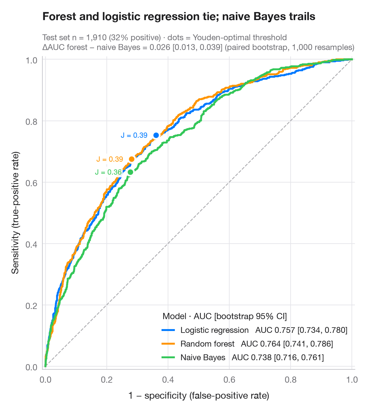
ROC 曲线描绘随着决策阈值由严到宽变化时,灵敏度相对于 1 − 特异度的变化轨迹。对角线相当于抛硬币;曲线越贴近左上角越好。AUC 是随机抽取的一个阳性样本得分高于随机抽取的一个阴性样本的概率;其 95% 区间来自对测试集的 1,000 次自助重抽样,并用配对自助法比较最优和最弱的模型。每条曲线上的点是使 Youden's J = 灵敏度 + 特异度 − 1 最大化的阈值。
数据为 Fair 婚外情调查的 6,366 名受访者(sm.datasets.fair),按 70/30 划分为训练集和测试集。来自 scikit-learn 的 logistic 回归、随机森林和朴素贝叶斯模型预测受访者是否报告有过婚外情;曲线和 AUC 由 roc_curve() 和 roc_auc_score() 计算。
代码及图中文字均为英文。
import matplotlib.pyplot as plt
import numpy as np
import statsmodels.api as sm
from sklearn.ensemble import RandomForestClassifier
from sklearn.linear_model import LogisticRegression
from sklearn.metrics import roc_auc_score, roc_curve
from sklearn.model_selection import train_test_split
from sklearn.naive_bayes import GaussianNB

# Data: predict any affair from the survey answers
df = sm.datasets.fair.load_pandas().data
X, y = df.drop(columns="affairs").to_numpy(), (df.affairs > 0).astype(int).to_numpy()
X_tr, X_te, y_tr, y_te = train_test_split(X, y, test_size=0.3, stratify=y, random_state=1)

models = {"Logistic regression": LogisticRegression(max_iter=1000),
          "Random forest": RandomForestClassifier(300, min_samples_leaf=20, random_state=1),
          "Naive Bayes": GaussianNB()}
palette = ["#007AFF", "#FF9500", "#34C759"]
rng = np.random.default_rng(42)
boot = [rng.integers(0, len(y_te), len(y_te)) for _ in range(1000)]

fig, ax = plt.subplots(figsize=(7, 6.4))
ax.plot([0, 1], [0, 1], color="#AEAEB2", lw=1, ls="--")
scores = {}
for (name, clf), c in zip(models.items(), palette):
    score = scores[name] = clf.fit(X_tr, y_tr).predict_proba(X_te)[:, 1]
    fpr, tpr, thr = roc_curve(y_te, score)
    auc = roc_auc_score(y_te, score)
    lo, hi = np.percentile([roc_auc_score(y_te[b], score[b]) for b in boot], [2.5, 97.5])
    ax.plot(fpr, tpr, color=c, lw=2.2, label=f"{name}   AUC {auc:.3f} [{lo:.3f}, {hi:.3f}]")
    # Youden's J: threshold that maximises TPR − FPR
    j = np.argmax(tpr - fpr)
    ax.scatter(fpr[j], tpr[j], s=70, color=c, edgecolor="white", lw=2, zorder=5)
    ax.annotate(f"J = {tpr[j] - fpr[j]:.2f}", (fpr[j], tpr[j]), xytext=(-10, 0),
                textcoords="offset points", fontsize=8.5, color=c, ha="right", va="center",
                bbox=dict(boxstyle="round,pad=0.15", fc="white", ec="none", alpha=0.9))

# Paired bootstrap: is the best model really better than the weakest?
a, b = scores["Random forest"], scores["Naive Bayes"]
diff = [roc_auc_score(y_te[i], a[i]) - roc_auc_score(y_te[i], b[i]) for i in boot]
d_lo, d_hi = np.percentile(diff, [2.5, 97.5])

ax.set_xlim(-0.01, 1.01); ax.set_ylim(-0.01, 1.01); ax.set_aspect("equal")
ax.grid(axis="x")
ax.set_xlabel("1 − specificity (false-positive rate)")
ax.set_ylabel("Sensitivity (true-positive rate)")
ax.legend(loc="lower right", title="Model · AUC [bootstrap 95% CI]", alignment="left",
          handlelength=1.4, fontsize=9.5)
ax.set_title("Forest and logistic regression tie; naive Bayes trails", pad=42)
ax.text(0, 1.02, f"Test set n = {len(y_te):,} ({y_te.mean():.0%} positive) · dots = Youden-optimal threshold\n"
        f"ΔAUC forest − naive Bayes = {roc_auc_score(y_te, a) - roc_auc_score(y_te, b):.3f} "
        f"[{d_lo:.3f}, {d_hi:.3f}] (paired bootstrap, 1,000 resamples)",
        transform=ax.transAxes, fontsize=9.5, color="#6E6E73")
plt.show()
图表使用了可选的 PyStatlas 样式:添加 plt.style.use("pystatlas.mplstyle") 即可完全还原其外观。
数据来源
- Redbook survey of married women, 1974 (Fair's affairs data). Fair, R. C. (1978). A theory of extramarital affairs. Journal of Political Economy, 86(1), 45–61. https://doi.org/10.1086/260646
Data from the 1974 Redbook magazine survey; distributed with statsmodels (sm.datasets.fair) with the author's permission.
这些示例用于说明统计方法。图表标题描述的是该图在这些特定数据中呈现的内容——这些数据往往样本较小、年代较早或并不完整——而不是作者对实质问题的立场。关于解释、背景和数据质量,请以此处引用的原始来源为准。
如何引用
PyStatlas 由 Thierry Warin 创建并维护。如果它对你的工作有所帮助,敬请引用。
Warin, T. (2026). ROC curves. In PyStatlas: A Python Gallery of Statistical Graphics for the Social Sciences. https://warint.github.io/pystatlas/model-diagnostics/roc-curve/
@misc{warin2026statlas,
  author       = {Warin, Thierry},
  title        = {PyStatlas: A Python Gallery of Statistical Graphics for the Social Sciences},
  year         = {2026},
  howpublished = {\url{https://warint.github.io/pystatlas/}},
  note         = {Source code: https://github.com/warint/pystatlas}
}