ROC curves — PyStatlas: A Python Gallery of Statistical Graphics for the Social Sciences

Warin, Thierry

ROC 曲線

3つの分類器を ROC 曲線、ブートストラップ 95% 信頼区間付きの AUC、ユーデン点で比較します。

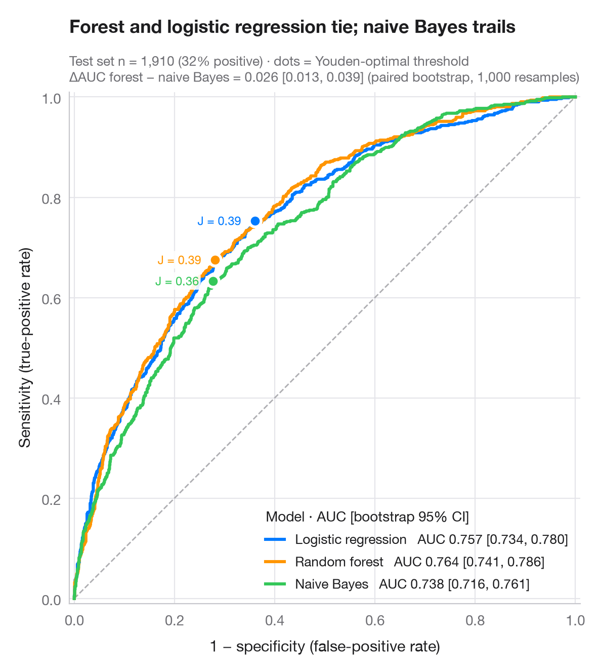
ROC 曲線は、判定の閾値を厳しい側から緩い側へ動かしたときの、感度と 1 − 特異度の関係をたどったものです。対角線はコイン投げに相当し、曲線が左上の角に近いほど優れています。AUC は、無作為に選んだ陽性例が無作為に選んだ陰性例より高いスコアを得る確率です。その 95% 信頼区間はテストセットの 1,000 回のブートストラップ再標本化から求め、対応のあるブートストラップで最良と最弱のモデルを比較しています。各曲線上の点は、ユーデンの J = 感度 + 特異度 − 1 を最大にする閾値です。

データはフェアの婚外関係調査の回答者 6,366 人（sm.datasets.fair）で、訓練用とテスト用に 70/30 で分割しています。scikit-learn のロジスティック回帰、ランダムフォレスト、ナイーブベイズの各モデルで、回答者が婚外関係を報告したかどうかを予測しています。曲線と AUC は roc_curve() と roc_auc_score() で求めています。

コードおよび図中のテキストは英語です。

roc-curve.py · 54 行

ダウンロード GitHub

import matplotlib.pyplot as plt
import numpy as np
import statsmodels.api as sm
from sklearn.ensemble import RandomForestClassifier
from sklearn.linear_model import LogisticRegression
from sklearn.metrics import roc_auc_score, roc_curve
from sklearn.model_selection import train_test_split
from sklearn.naive_bayes import GaussianNB

# Data: predict any affair from the survey answers
df = sm.datasets.fair.load_pandas().data
X, y = df.drop(columns="affairs").to_numpy(), (df.affairs > 0).astype(int).to_numpy()
X_tr, X_te, y_tr, y_te = train_test_split(X, y, test_size=0.3, stratify=y, random_state=1)

models = {"Logistic regression": LogisticRegression(max_iter=1000),
          "Random forest": RandomForestClassifier(300, min_samples_leaf=20, random_state=1),
          "Naive Bayes": GaussianNB()}
palette = ["#007AFF", "#FF9500", "#34C759"]
rng = np.random.default_rng(42)
boot = [rng.integers(0, len(y_te), len(y_te)) for _ in range(1000)]

fig, ax = plt.subplots(figsize=(7, 6.4))
ax.plot([0, 1], [0, 1], color="#AEAEB2", lw=1, ls="--")
scores = {}
for (name, clf), c in zip(models.items(), palette):
    score = scores[name] = clf.fit(X_tr, y_tr).predict_proba(X_te)[:, 1]
    fpr, tpr, thr = roc_curve(y_te, score)
    auc = roc_auc_score(y_te, score)
    lo, hi = np.percentile([roc_auc_score(y_te[b], score[b]) for b in boot], [2.5, 97.5])
    ax.plot(fpr, tpr, color=c, lw=2.2, label=f"{name}   AUC {auc:.3f} [{lo:.3f}, {hi:.3f}]")
    # Youden's J: threshold that maximises TPR − FPR
    j = np.argmax(tpr - fpr)
    ax.scatter(fpr[j], tpr[j], s=70, color=c, edgecolor="white", lw=2, zorder=5)
    ax.annotate(f"J = {tpr[j] - fpr[j]:.2f}", (fpr[j], tpr[j]), xytext=(-10, 0),
                textcoords="offset points", fontsize=8.5, color=c, ha="right", va="center",
                bbox=dict(boxstyle="round,pad=0.15", fc="white", ec="none", alpha=0.9))

# Paired bootstrap: is the best model really better than the weakest?
a, b = scores["Random forest"], scores["Naive Bayes"]
diff = [roc_auc_score(y_te[i], a[i]) - roc_auc_score(y_te[i], b[i]) for i in boot]
d_lo, d_hi = np.percentile(diff, [2.5, 97.5])

ax.set_xlim(-0.01, 1.01); ax.set_ylim(-0.01, 1.01); ax.set_aspect("equal")
ax.grid(axis="x")
ax.set_xlabel("1 − specificity (false-positive rate)")
ax.set_ylabel("Sensitivity (true-positive rate)")
ax.legend(loc="lower right", title="Model · AUC [bootstrap 95% CI]", alignment="left",
          handlelength=1.4, fontsize=9.5)
ax.set_title("Forest and logistic regression tie; naive Bayes trails", pad=42)
ax.text(0, 1.02, f"Test set n = {len(y_te):,} ({y_te.mean():.0%} positive) · dots = Youden-optimal threshold\n"
        f"ΔAUC forest − naive Bayes = {roc_auc_score(y_te, a) - roc_auc_score(y_te, b):.3f} "
        f"[{d_lo:.3f}, {d_hi:.3f}] (paired bootstrap, 1,000 resamples)",
        transform=ax.transAxes, fontsize=9.5, color="#6E6E73")
plt.show()

図にはオプションの PyStatlas スタイルを使用しています。同じ見た目にするには plt.style.use("pystatlas.mplstyle") を追加してください。

データの出典

Redbook survey of married women, 1974 (Fair's affairs data). Fair, R. C. (1978). A theory of extramarital affairs. Journal of Political Economy, 86(1), 45–61. https://doi.org/10.1086/260646
Data from the 1974 Redbook magazine survey; distributed with statsmodels (sm.datasets.fair) with the author's permission.

これらの例は統計手法を説明するためのものです。図のタイトルは、この特定のデータ（多くは小規模で、古く、部分的な標本）で図が示す内容を述べたものであり、実質的な問いに対する著者の立場ではありません。解釈、背景、データの質については、ここに挙げた元の出典を参照してください。

引用方法

PyStatlas は Thierry Warin が作成・運営しています。研究や業務に役立った場合は、ぜひ引用してください。

Warin, T. (2026). ROC curves. In PyStatlas: A Python Gallery of Statistical Graphics for the Social Sciences. https://warint.github.io/pystatlas/model-diagnostics/roc-curve/

@misc{warin2026statlas,
  author       = {Warin, Thierry},
  title        = {PyStatlas: A Python Gallery of Statistical Graphics for the Social Sciences},
  year         = {2026},
  howpublished = {\url{https://warint.github.io/pystatlas/}},
  note         = {Source code: https://github.com/warint/pystatlas}
}