校准图
按十分位分组的预测风险与观测风险,附 Wilson 置信区间、预测值直方图和 Brier 分数。
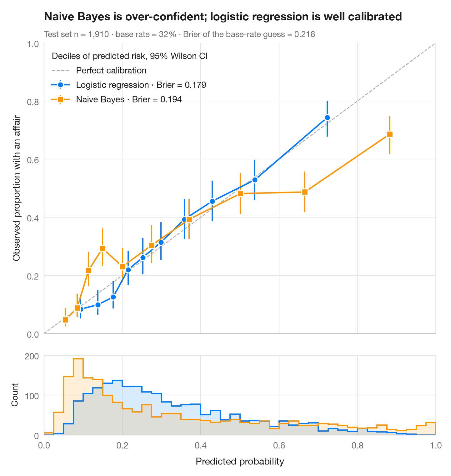
一个模型可以很好地对样本排序(AUC 高),却仍然给出错误的概率。可靠性图正是用来检验这一点的:测试样本按预测风险分为十个十分位组,每组的平均预测值与观测事件率相对照,并附 95% Wilson 区间。校准良好的模型落在对角线上;点位于对角线下方意味着模型过度自信。下方的直方图展示预测值的实际分布位置。
数据为 Fair 婚外情调查(sm.datasets.fair),按 70/30 划分。比较来自 scikit-learn 的 logistic 回归和高斯朴素贝叶斯模型;Brier 分数(brier_score_loss,越低越好)概括概率预测的准确度,区间由 proportion_confint(method="wilson") 计算。
代码及图中文字均为英文。
import matplotlib.pyplot as plt
import numpy as np
import pandas as pd
import statsmodels.api as sm
from sklearn.linear_model import LogisticRegression
from sklearn.metrics import brier_score_loss
from sklearn.model_selection import train_test_split
from sklearn.naive_bayes import GaussianNB
from statsmodels.stats.proportion import proportion_confint

df = sm.datasets.fair.load_pandas().data
X, y = df.drop(columns="affairs").to_numpy(), (df.affairs > 0).astype(int).to_numpy()
X_tr, X_te, y_tr, y_te = train_test_split(X, y, test_size=0.3, stratify=y, random_state=1)
models = {"Logistic regression": (LogisticRegression(max_iter=1000), "#007AFF", "o"),
          "Naive Bayes": (GaussianNB(), "#FF9500", "s")}

fig, (ax, axh) = plt.subplots(2, 1, figsize=(7, 7.4), sharex=True,
                              gridspec_kw=dict(height_ratios=[4, 1.1], hspace=0.05))
ax.plot([0, 1], [0, 1], color="#AEAEB2", lw=1, ls="--", label="Perfect calibration")
bins = np.linspace(0, 1, 41)
for name, (clf, c, mk) in models.items():
    p = clf.fit(X_tr, y_tr).predict_proba(X_te)[:, 1]
    # Group predictions into deciles of predicted risk
    tab = (pd.DataFrame({"p": p, "y": y_te})
             .assign(bin=lambda d: pd.qcut(d.p, 10, labels=False, duplicates="drop"))
             .groupby("bin").agg(pred=("p", "mean"), obs=("y", "mean"), k=("y", "sum"), n=("y", "size")))
    lo, hi = proportion_confint(tab.k, tab.n, method="wilson")
    ax.errorbar(tab.pred, tab.obs, yerr=[tab.obs - lo, hi - tab.obs], fmt=mk + "-", color=c,
                ms=7, mec="white", mew=1.2, lw=1.6, capsize=0, elinewidth=1.4,
                label=f"{name} · Brier = {brier_score_loss(y_te, p):.3f}")
    axh.hist(p, bins=bins, color=c, alpha=0.15, lw=0)
    axh.hist(p, bins=bins, color=c, histtype="step", lw=1.4)

ax.set_xlim(0, 1); ax.set_ylim(0, 1); ax.set_aspect("auto")
ax.grid(axis="x")
ax.set_ylabel("Observed proportion with an affair")
ax.legend(loc="upper left", alignment="left", title="Deciles of predicted risk, 95% Wilson CI")
axh.set_xlabel("Predicted probability")
axh.set_ylabel("Count", fontsize=10)
axh.grid(axis="x")
ax.set_title("Naive Bayes is over-confident; logistic regression is well calibrated", pad=26)
ax.text(0, 1.02, f"Test set n = {len(y_te):,} · base rate = {y_te.mean():.0%} · "
        f"Brier of the base-rate guess = {y_te.mean() * (1 - y_te.mean()):.3f}",
        transform=ax.transAxes, fontsize=9.5, color="#6E6E73")
plt.show()
图表使用了可选的 PyStatlas 样式:添加 plt.style.use("pystatlas.mplstyle") 即可完全还原其外观。
数据来源
- Redbook survey of married women, 1974 (Fair's affairs data). Fair, R. C. (1978). A theory of extramarital affairs. Journal of Political Economy, 86(1), 45–61. https://doi.org/10.1086/260646
Data from the 1974 Redbook magazine survey; distributed with statsmodels (sm.datasets.fair) with the author's permission.
这些示例用于说明统计方法。图表标题描述的是该图在这些特定数据中呈现的内容——这些数据往往样本较小、年代较早或并不完整——而不是作者对实质问题的立场。关于解释、背景和数据质量,请以此处引用的原始来源为准。
如何引用
PyStatlas 由 Thierry Warin 创建并维护。如果它对你的工作有所帮助,敬请引用。
Warin, T. (2026). Calibration plot. In PyStatlas: A Python Gallery of Statistical Graphics for the Social Sciences. https://warint.github.io/pystatlas/model-diagnostics/calibration-plot/
@misc{warin2026statlas,
  author       = {Warin, Thierry},
  title        = {PyStatlas: A Python Gallery of Statistical Graphics for the Social Sciences},
  year         = {2026},
  howpublished = {\url{https://warint.github.io/pystatlas/}},
  note         = {Source code: https://github.com/warint/pystatlas}
}