残差诊断
线性模型经典的 2 × 2 诊断图——线性、正态性、方差与杠杆值。
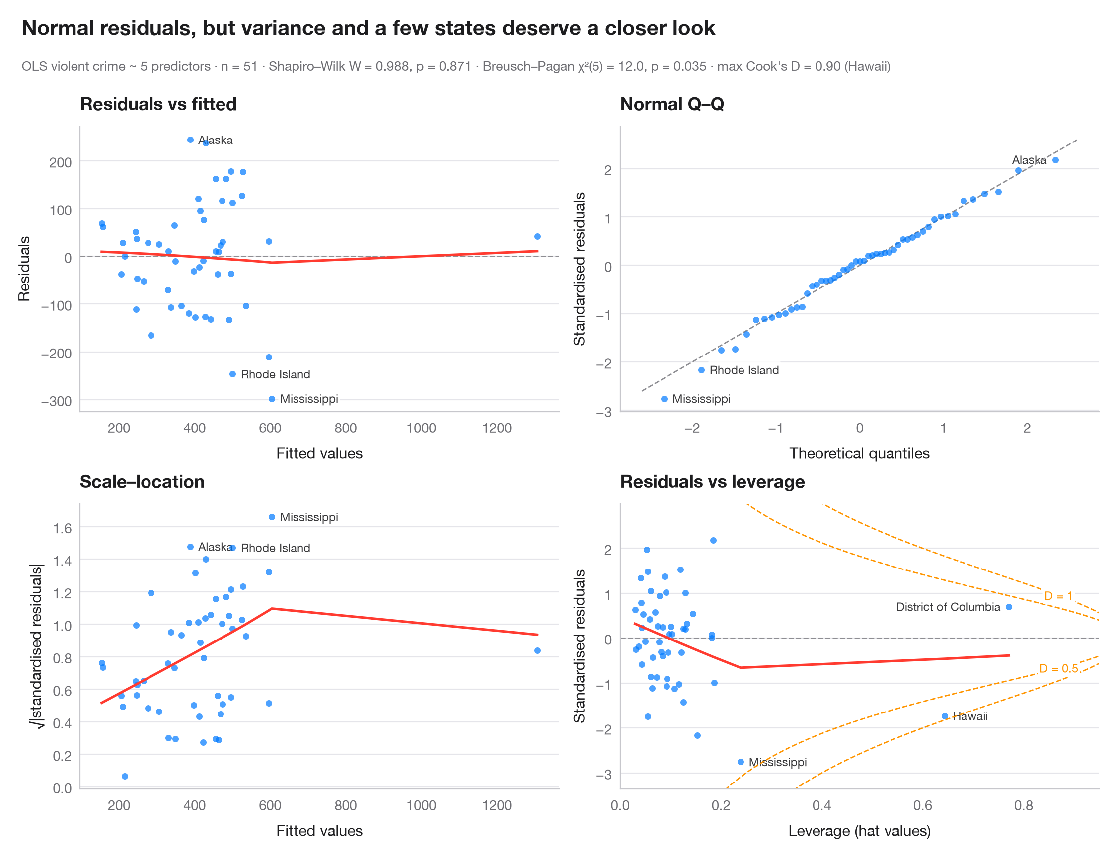
残差的四种视图回答四个问题。残差与拟合值:关系是否为线性(LOWESS 曲线是否平坦)?正态 Q–Q 图:残差是否近似正态(点是否落在直线上)?尺度–位置图:离散程度是否恒定(曲线是否平坦)?残差与杠杆值:是否有观测值在牵引拟合,即落在 Cook 距离虚线等值线之外?每个子图都标注了三个最极端的观测值,正式检验结果列于副标题。
模型是基于 sm.datasets.statecrime 中美国 50 个州 + 哥伦比亚特区的暴力犯罪回归。所有结果均来自 statsmodels 的 get_influence(),另用 lowess() 绘制平滑曲线,并使用 het_breuschpagan() 和 scipy.stats.shapiro()。
代码及图中文字均为英文。
import matplotlib.pyplot as plt
import numpy as np
import statsmodels.api as sm
import statsmodels.formula.api as smf
from scipy import stats
from statsmodels.nonparametric.smoothers_lowess import lowess
from statsmodels.stats.diagnostic import het_breuschpagan

df = sm.datasets.statecrime.load_pandas().data
model = smf.ols("violent ~ poverty + single + urban + hs_grad + white", data=df).fit()
infl = model.get_influence()
fitted, resid = model.fittedvalues, model.resid
std_r, lev, cook = infl.resid_studentized_internal, infl.hat_matrix_diag, infl.cooks_distance[0]
p = model.df_model + 1
top = np.argsort(-np.abs(std_r))[:3]                # 3 largest standardised residuals

fig, axes = plt.subplots(2, 2, figsize=(11, 7.6))
kw = dict(s=22, color="#007AFF", alpha=0.7, lw=0, zorder=2)
smooth = dict(color="#FF3B30", lw=1.8)

def label(ax, x, y, idx):
    lo, hi = ax.get_xlim()
    for i in idx:                                   # text on the side with more room
        right = (x[i] - lo) / (hi - lo) < 0.75
        ax.annotate(df.index[i], (x[i], y[i]), xytext=(6 if right else -6, 0),
                    textcoords="offset points", ha="left" if right else "right",
                    va="center", fontsize=8.5, color="#3A3A3C", zorder=1,
                    bbox=dict(boxstyle="round,pad=0.15", fc="white", ec="none", alpha=0.85))


# 1. Residuals vs fitted
ax = axes[0, 0]
ax.axhline(0, color="#8E8E93", lw=1, ls="--")
ax.scatter(fitted, resid, **kw)
ax.plot(*lowess(resid, fitted, frac=1, it=0).T, **smooth)
label(ax, fitted.values, resid.values, top)
ax.set(title="Residuals vs fitted", xlabel="Fitted values", ylabel="Residuals")

# 2. Normal Q-Q of standardised residuals
ax = axes[0, 1]
order = np.argsort(std_r)
theo = stats.norm.ppf((np.arange(1, len(std_r) + 1) - 0.5) / len(std_r))
ax.plot([-2.6, 2.6], [-2.6, 2.6], color="#8E8E93", lw=1, ls="--")
ax.scatter(theo, std_r[order], **kw)
rank = {i: k for k, i in enumerate(order)}
label(ax, {i: theo[rank[i]] for i in top}, std_r, top)
ax.set(title="Normal Q–Q", xlabel="Theoretical quantiles", ylabel="Standardised residuals")

# 3. Scale-location
ax = axes[1, 0]
root = np.sqrt(np.abs(std_r))
ax.scatter(fitted, root, **kw)
ax.plot(*lowess(root, fitted, frac=1, it=0).T, **smooth)
label(ax, fitted.values, np.abs(root), top)
ax.set(title="Scale–location", xlabel="Fitted values", ylabel="√|standardised residuals|")

# 4. Residuals vs leverage with Cook's distance contours
ax = axes[1, 1]
ax.axhline(0, color="#8E8E93", lw=1, ls="--")
ax.scatter(lev, std_r, **kw)
ax.plot(*lowess(std_r, lev, frac=1, it=0).T, **smooth)
ylim = (std_r.min() - 0.6, std_r.max() + 0.8)
h = np.linspace(0.01, 0.95, 300)
for D in (0.5, 1):
    r = np.sqrt(D * p * (1 - h) / h)
    ax.plot(h, r, color="#FF9500", lw=1, ls="--"); ax.plot(h, -r, color="#FF9500", lw=1, ls="--")
    sign = 1 if D == 1 else -1                       # label D = 1 above, D = 0.5 below
    ax.text(0.87, sign * np.sqrt(D * p * 0.13 / 0.87), f"D = {D}", color="#FF9500", fontsize=8.5,
            ha="center", va="center", bbox=dict(boxstyle="round,pad=0.15", fc="white", ec="none"))
ax.set_ylim(*ylim); ax.set_xlim(0, 0.95)
label(ax, lev, std_r, np.argsort(-cook)[:3])
ax.set(title="Residuals vs leverage", xlabel="Leverage (hat values)", ylabel="Standardised residuals")
for a in axes.flat:
    a.title.set_fontsize(12)

bp = het_breuschpagan(resid, model.model.exog)
sw = stats.shapiro(resid)
fig.text(0.01, 1.065, "Normal residuals, but variance and a few states deserve a closer look",
         fontsize=15, fontweight="semibold", va="bottom")
fig.text(0.01, 1.02, f"OLS violent crime ~ 5 predictors · n = {int(model.nobs)} · Shapiro–Wilk "
         f"W = {sw.statistic:.3f}, p = {sw.pvalue:.3f} · Breusch–Pagan χ²({p - 1:.0f}) = "
         f"{bp[0]:.1f}, p = {bp[1]:.3f} · max Cook's D = {cook.max():.2f} ({df.index[cook.argmax()]})",
         fontsize=9.5, color="#6E6E73", va="bottom")
plt.show()
图表使用了可选的 PyStatlas 样式:添加 plt.style.use("pystatlas.mplstyle") 即可完全还原其外观。
数据来源
- US state crime and social indicators, 2009. U.S. Census Bureau. Statistical Abstract of the United States, state tables for 2009 (crime rates from the FBI Uniform Crime Reporting program). https://www.statsmodels.org/stable/datasets/generated/statecrime.html
Compiled for statsmodels (sm.datasets.statecrime); public domain. See the statsmodels page for each variable's table and footnotes.
这些示例用于说明统计方法。图表标题描述的是该图在这些特定数据中呈现的内容——这些数据往往样本较小、年代较早或并不完整——而不是作者对实质问题的立场。关于解释、背景和数据质量,请以此处引用的原始来源为准。
如何引用
PyStatlas 由 Thierry Warin 创建并维护。如果它对你的工作有所帮助,敬请引用。
Warin, T. (2026). Residual diagnostics. In PyStatlas: A Python Gallery of Statistical Graphics for the Social Sciences. https://warint.github.io/pystatlas/model-diagnostics/residual-diagnostics/
@misc{warin2026statlas,
  author       = {Warin, Thierry},
  title        = {PyStatlas: A Python Gallery of Statistical Graphics for the Social Sciences},
  year         = {2026},
  howpublished = {\url{https://warint.github.io/pystatlas/}},
  note         = {Source code: https://github.com/warint/pystatlas}
}