Cross-table with standardized residuals
A contingency table as a heatmap, coloured by standardized residuals from independence.
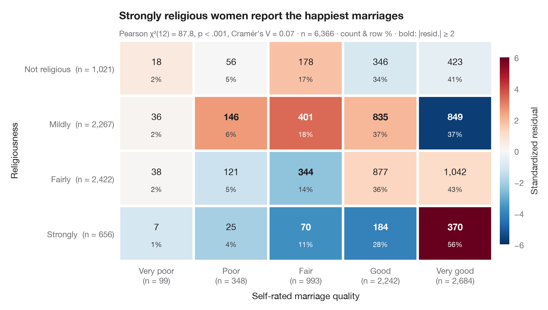
The Python counterpart of ggstats::ggtable(): the familiar cross-tab, but each
cell is coloured by its standardized (adjusted) residual — how many standard
errors the observed count sits above or below what independence would predict.
Under independence these residuals are roughly standard normal, so cells beyond
±2 (marked in bold) are the ones that make the χ² test significant. Each cell
prints the count and its row percentage; the margins give the totals.
Data are the 1974 Redbook survey bundled with statsmodels
(sm.datasets.fair): religiousness against self-rated marriage quality for 6,366
women. Expected counts come from scipy.stats.chi2_contingency; the residual is
(O − E) / √(E · (1 − row share) · (1 − column share)).
import matplotlib.pyplot as plt
import numpy as np
import pandas as pd
import statsmodels.api as sm
from matplotlib.colors import TwoSlopeNorm
from scipy import stats

# Data: religiousness (rows) × marriage rating (columns)
df = sm.datasets.fair.load_pandas().data
rel = df.religious.map({1: "Not religious", 2: "Mildly", 3: "Fairly", 4: "Strongly"})
rate = df.rate_marriage.map({1: "Very poor", 2: "Poor", 3: "Fair", 4: "Good", 5: "Very good"})
table = pd.crosstab(pd.Categorical(rel, ["Not religious", "Mildly", "Fairly", "Strongly"]),
                    pd.Categorical(rate, ["Very poor", "Poor", "Fair", "Good", "Very good"]))
obs = table.to_numpy()
n = obs.sum()

# Chi-squared test and adjusted (standardized) residuals
chi2, p, dof, exp = stats.chi2_contingency(obs, correction=False)
row_share, col_share = obs.sum(1, keepdims=True) / n, obs.sum(0, keepdims=True) / n
std_resid = (obs - exp) / np.sqrt(exp * (1 - row_share) * (1 - col_share))
row_pct = obs / obs.sum(1, keepdims=True) * 100
v = np.sqrt(chi2 / (n * (min(obs.shape) - 1)))

fig, ax = plt.subplots(figsize=(9, 5))
norm = TwoSlopeNorm(0, vmin=-6, vmax=6)
im = ax.imshow(std_resid, cmap="RdBu_r", norm=norm, aspect="auto")
for i in range(obs.shape[0]):
    for j in range(obs.shape[1]):
        strong = abs(std_resid[i, j]) >= 2
        ax.text(j, i - 0.12, f"{obs[i, j]:,}", ha="center", va="center", fontsize=11,
                fontweight="bold" if strong else "normal",
                color="white" if abs(std_resid[i, j]) > 3 else "#1D1D1F")
        ax.text(j, i + 0.2, f"{row_pct[i, j]:.0f}%", ha="center", va="center", fontsize=8.5,
                color="white" if abs(std_resid[i, j]) > 3 else "#3A3A3C")

# White gutters between cells and totals in the margins
ax.set_xticks(np.arange(-0.5, obs.shape[1]), minor=True)
ax.set_yticks(np.arange(-0.5, obs.shape[0]), minor=True)
ax.grid(which="minor", color="white", lw=3)
ax.grid(which="major", visible=False)
ax.tick_params(which="minor", length=0)
ax.set_xticks(range(obs.shape[1]), [f"{c}\n(n = {t:,})" for c, t in zip(table.columns, obs.sum(0))])
ax.set_yticks(range(obs.shape[0]), [f"{r}  (n = {t:,})" for r, t in zip(table.index, obs.sum(1))])
for s in ax.spines.values():
    s.set_visible(False)
ax.set_xlabel("Self-rated marriage quality")
ax.set_ylabel("Religiousness")

cb = fig.colorbar(im, ax=ax, shrink=0.85, pad=0.02, ticks=[-6, -4, -2, 0, 2, 4, 6])
cb.set_label("Standardized residual", color="#3A3A3C")
cb.outline.set_visible(False)
ax.set_title("Strongly religious women report the happiest marriages", pad=26)
ax.text(0, 1.02, f"Pearson χ²({dof}) = {chi2:.1f}, p < .001, Cramér's V = {v:.2f} · n = {n:,} · "
        "count & row % · bold: |resid.| ≥ 2", transform=ax.transAxes,
        fontsize=9.5, color="#6E6E73")
plt.show()
Figures use the optional PyStatlas style: add plt.style.use("pystatlas.mplstyle") to match the look exactly.
Data source
- Redbook survey of married women, 1974 (Fair's affairs data). Fair, R. C. (1978). A theory of extramarital affairs. Journal of Political Economy, 86(1), 45–61. https://doi.org/10.1086/260646
Data from the 1974 Redbook magazine survey; distributed with statsmodels (sm.datasets.fair) with the author's permission.
The examples illustrate statistical methods. Their titles describe what each figure shows in these particular data — often a small, dated or partial sample — not the author's position on the substantive question. For interpretation, context and data quality, rely on the original sources cited here.
How to cite
PyStatlas is created and maintained by Thierry Warin. If it helped your work, please cite it.
Warin, T. (2026). Cross-table with standardized residuals. In PyStatlas: A Python Gallery of Statistical Graphics for the Social Sciences. https://warint.github.io/pystatlas/proportions-surveys/crosstab-residuals/
@misc{warin2026statlas,
  author       = {Warin, Thierry},
  title        = {PyStatlas: A Python Gallery of Statistical Graphics for the Social Sciences},
  year         = {2026},
  howpublished = {\url{https://warint.github.io/pystatlas/}},
  note         = {Source code: https://github.com/warint/pystatlas}
}More in Proportions & surveys
Diverging Likert chart
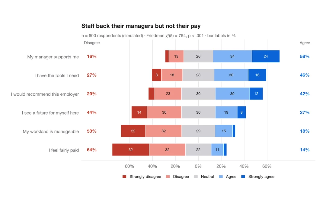
Five-point Likert items as diverging stacked bars centred on the neutral answer.
ggstats::gglikert()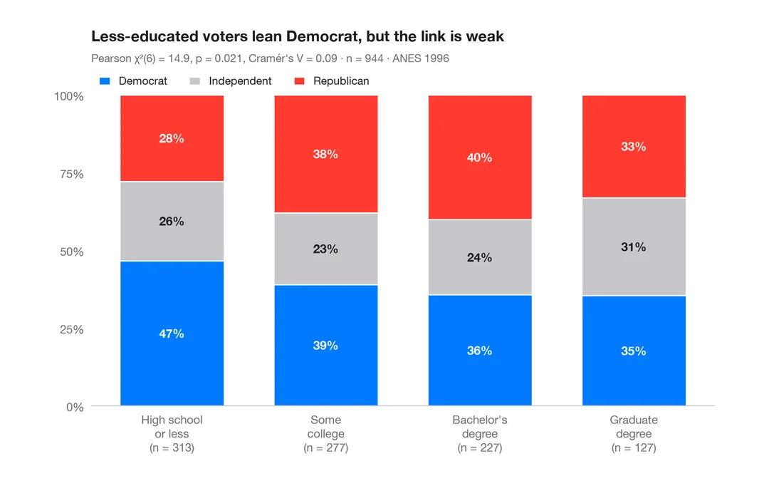
Stacked proportions by group
100% stacked bars with percentage labels, n per bar, chi-squared test and Cramér's V.
ggstatsplot::ggbarstats()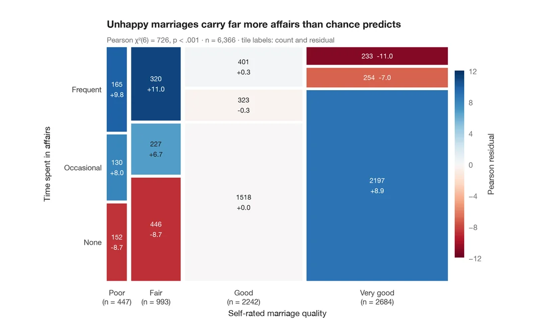
Mosaic plot with Pearson residuals
Tile areas proportional to cell counts, shaded by Pearson residuals from independence.
vcd::mosaic(shade = TRUE)