带标准化残差的交叉表
以热图呈现的列联表,按相对于独立性的标准化残差着色。
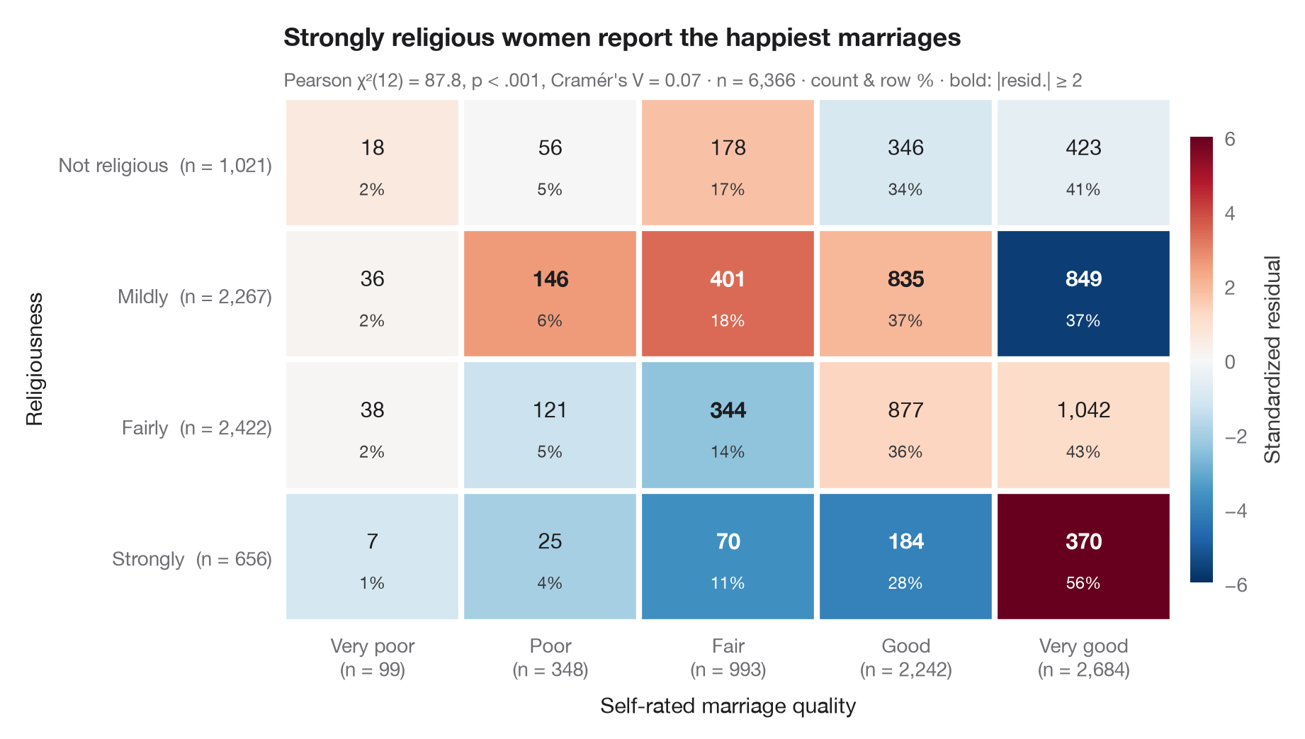
ggstats::ggtable() 的 Python 版本:熟悉的交叉表,但每个单元格按其标准化(调整)残差着色——即观测频数高于或低于独立假设预测值多少个标准误。在独立假设下,这些残差近似服从标准正态分布,因此超过 ±2 的单元格(以粗体标出)正是使 χ² 检验显著的那些。每个单元格显示频数及其行百分比;边际给出合计。
数据为 statsmodels 自带的 1974 年 Redbook 调查(sm.datasets.fair):6,366 名女性的宗教虔诚度与自评婚姻质量。期望频数由 scipy.stats.chi2_contingency 计算;残差为 (O − E) / √(E · (1 − 行比例) · (1 − 列比例))。
代码及图中文字均为英文。
import matplotlib.pyplot as plt
import numpy as np
import pandas as pd
import statsmodels.api as sm
from matplotlib.colors import TwoSlopeNorm
from scipy import stats

# Data: religiousness (rows) × marriage rating (columns)
df = sm.datasets.fair.load_pandas().data
rel = df.religious.map({1: "Not religious", 2: "Mildly", 3: "Fairly", 4: "Strongly"})
rate = df.rate_marriage.map({1: "Very poor", 2: "Poor", 3: "Fair", 4: "Good", 5: "Very good"})
table = pd.crosstab(pd.Categorical(rel, ["Not religious", "Mildly", "Fairly", "Strongly"]),
                    pd.Categorical(rate, ["Very poor", "Poor", "Fair", "Good", "Very good"]))
obs = table.to_numpy()
n = obs.sum()

# Chi-squared test and adjusted (standardized) residuals
chi2, p, dof, exp = stats.chi2_contingency(obs, correction=False)
row_share, col_share = obs.sum(1, keepdims=True) / n, obs.sum(0, keepdims=True) / n
std_resid = (obs - exp) / np.sqrt(exp * (1 - row_share) * (1 - col_share))
row_pct = obs / obs.sum(1, keepdims=True) * 100
v = np.sqrt(chi2 / (n * (min(obs.shape) - 1)))

fig, ax = plt.subplots(figsize=(9, 5))
norm = TwoSlopeNorm(0, vmin=-6, vmax=6)
im = ax.imshow(std_resid, cmap="RdBu_r", norm=norm, aspect="auto")
for i in range(obs.shape[0]):
    for j in range(obs.shape[1]):
        strong = abs(std_resid[i, j]) >= 2
        ax.text(j, i - 0.12, f"{obs[i, j]:,}", ha="center", va="center", fontsize=11,
                fontweight="bold" if strong else "normal",
                color="white" if abs(std_resid[i, j]) > 3 else "#1D1D1F")
        ax.text(j, i + 0.2, f"{row_pct[i, j]:.0f}%", ha="center", va="center", fontsize=8.5,
                color="white" if abs(std_resid[i, j]) > 3 else "#3A3A3C")

# White gutters between cells and totals in the margins
ax.set_xticks(np.arange(-0.5, obs.shape[1]), minor=True)
ax.set_yticks(np.arange(-0.5, obs.shape[0]), minor=True)
ax.grid(which="minor", color="white", lw=3)
ax.grid(which="major", visible=False)
ax.tick_params(which="minor", length=0)
ax.set_xticks(range(obs.shape[1]), [f"{c}\n(n = {t:,})" for c, t in zip(table.columns, obs.sum(0))])
ax.set_yticks(range(obs.shape[0]), [f"{r}  (n = {t:,})" for r, t in zip(table.index, obs.sum(1))])
for s in ax.spines.values():
    s.set_visible(False)
ax.set_xlabel("Self-rated marriage quality")
ax.set_ylabel("Religiousness")

cb = fig.colorbar(im, ax=ax, shrink=0.85, pad=0.02, ticks=[-6, -4, -2, 0, 2, 4, 6])
cb.set_label("Standardized residual", color="#3A3A3C")
cb.outline.set_visible(False)
ax.set_title("Strongly religious women report the happiest marriages", pad=26)
ax.text(0, 1.02, f"Pearson χ²({dof}) = {chi2:.1f}, p < .001, Cramér's V = {v:.2f} · n = {n:,} · "
        "count & row % · bold: |resid.| ≥ 2", transform=ax.transAxes,
        fontsize=9.5, color="#6E6E73")
plt.show()
图表使用了可选的 PyStatlas 样式:添加 plt.style.use("pystatlas.mplstyle") 即可完全还原其外观。
数据来源
- Redbook survey of married women, 1974 (Fair's affairs data). Fair, R. C. (1978). A theory of extramarital affairs. Journal of Political Economy, 86(1), 45–61. https://doi.org/10.1086/260646
Data from the 1974 Redbook magazine survey; distributed with statsmodels (sm.datasets.fair) with the author's permission.
这些示例用于说明统计方法。图表标题描述的是该图在这些特定数据中呈现的内容——这些数据往往样本较小、年代较早或并不完整——而不是作者对实质问题的立场。关于解释、背景和数据质量,请以此处引用的原始来源为准。
如何引用
PyStatlas 由 Thierry Warin 创建并维护。如果它对你的工作有所帮助,敬请引用。
Warin, T. (2026). Cross-table with standardized residuals. In PyStatlas: A Python Gallery of Statistical Graphics for the Social Sciences. https://warint.github.io/pystatlas/proportions-surveys/crosstab-residuals/
@misc{warin2026statlas,
  author       = {Warin, Thierry},
  title        = {PyStatlas: A Python Gallery of Statistical Graphics for the Social Sciences},
  year         = {2026},
  howpublished = {\url{https://warint.github.io/pystatlas/}},
  note         = {Source code: https://github.com/warint/pystatlas}
}